Custom mixed finite-element SIMPLE solver

Dr. Jaydeep Deshpande September 10, 2026

Numerical experiments on Face enriched P1/P0 or Q1/Q0 FEM function space

The article describes a SIMPLE-type incompressible-flow solver built with mixed finite elements discretization. The central idea is to use a continuous velocity space enriched by shared face degrees of freedom, pair it with one discontinuous pressure unknown per cell, and exploit that topology to build a cheap pressure-correction operator. The objective was to document a useful numerical experiment, in which a mixed FE formulation can retain a local cellwise continuity equation, avoid pressure-stabilization devices such as PSPG or Rhie-Chow interpolation, and still admit a very cheap SIMPLE-like pressure correction.

1. Why a mixed finite-element SIMPLE solver?

For incompressible flow, the familiar numerical tension is between velocity-pressure stability, local mass balance, robustness at high Reynolds number, and cost. A collocated finite-volume method is attractive because both the velocity and pressure unknowns are cell-centred. A collocated formulation much like equal order finite element pairs, runs into the inf-sup problem: in short the pressure -velocity discretization is rank deficient and thus its pressure to velocity relationship is not adequately represented. The problem is circumvented through the addition of dissipation terms like Rhie-Chow interpolation, Brezzi-Pitkaranta term or pressure stabilized Petrov-Galerkin (PSPG) term to the pressure-pressure block of incompressible Navier-Stokes. Staggered FV discretizations which treat pressure at the cell center and velocity as constant flux face variables naturally avoid the rank-deficiency and are able to provide a formulation that conserves mass accurately. However, an ‘unstructured FV staggering’ is still not a solved problem. What even does staggering mean in an unstructured sense? In this respect finite-elements provide a cleaner approach with mixed elements like P2-P1 (quadratic velocity, linear pressure) which can be used on unstructured meshes without the rank deficiency. However these implementations are typically implemented in FEM softwares in continuous galerkin format, which does not provide local mass balance since the pressure test function is continuous. As against this discontinuous P2-P1 formulations provide the local mass balance but are extremely heavy to run. The majority of FEM literature though is quite focused on monolithic solvers which do not solve Navier Stokes in segregated manner. This results in even matrix free FEM solvers reaching memory requirements close to 15-20 GB/ million cells. Such a big memory bandwidth creates a slow solver. A straightforward solution could be to use a low-order continuous finite-element pair continuous linear (P1) velocity with discontinuous zeroth order (P0) pressure. Unfortunately, though this function space is mixed, it is not inf-sup stable.

We thus started from a third option derived originally by Farrell et al (2019) for the Augmented Lagrangian Preconditioner.

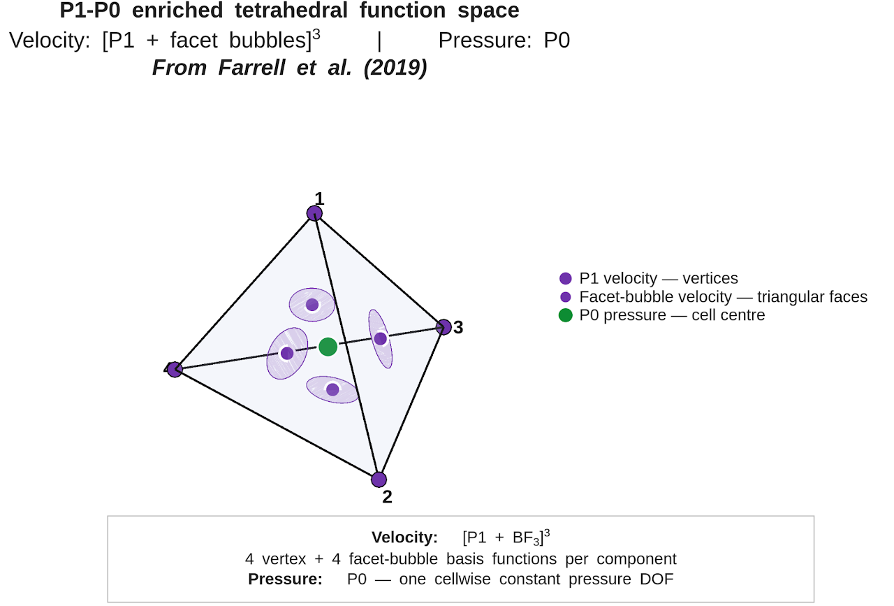
The velocity remains globally continuous, but it is enriched with velocity degrees of freedom associated with element faces. The pressure is discontinuous and constant within each cell, which allows the pressure test function to test local mass balance (see the next section). Additionally the topology appears surprisingly close to a staggered method: pressure lives in cells, while the additional shared velocity modes help in providing the discrete divergence that couples with neighbouring cells without adding an artificial pressure-dissipation term.

Governing incompressible momentum and continuity equations

Convection can be treated centrally, or streamline-upwind/Petrov-Galerkin stabilization can be added when desired. Crucially, upwinding acts through the momentum discretization; pressure is not stabilized by a PSPG term, and the solver does not need a Rhie-Chow-style pressure filter.

Note that this tetrahedral element that motivated the original NodalS solver is the face-bubble-enriched pair discussed by Farrell, Mitchell and Wechsung in their 2019 high-Reynolds-number preconditioning work and is not the invention of the current author. More precisely, the formulation enriches all three components of P1 velocity with cubic facet bubbles and pairs the result with discontinuous P0 pressure.

Original tetrahedral NodalS velocity-pressure pair

The face bubble is just an extra shared velocity degree of freedom attached to a face and is able to participate int typical FEM continuous galerkin assembly. However note that its contribution goes to zero at the other face nodes, thus it provides an added a degree of independence to the solver for attacking the face contributions that are shared exactly between 2 cells, unlike the nodes which are shared with a large number of neighboring cells. This feature is also later preserved in the hexahedral analogue.

2. Why discontinuous cell pressure is useful

The pressure space contains one constant test function per cell. Since pressure acts like the lagrange multiplier enforcing the continuity/mass balance, the pressure test function is utilized on the continuity equation assembly. This has an immediate consequence for continuity: choosing the pressure test function to be one on a particular element and zero elsewhere enforces the integrated divergence equation on that element in a manner which closer to how traditional FVM does.

The Q0/P0 pressure equation is one integrated mass-balance equation per cell

This is the sense in which the method is locally conservative. Note that it does not say that every pointwise or higher-order moment of divergence vanishes inside a cell. It says that the net flux through the cell boundary is zero to the accuracy of the finite-element quadrature and numerical boundary traces.

At the same time, the velocity field is continuous across an interior face. There is therefore one shared velocity trace rather than two independent traces, which is convenient for a flux interpretation. The resulting formulation combines a continuous Galerkin velocity field with a discontinuous cell pressure without turning the entire method into a heavy DG solver.

Schematic mixed weak form used by the solver

3. This function space is naturally useful for SIMPLE

After discretization and linearization, the incompressible problem has the standard saddle-point structure.

Equivalent block form of the discrete mixed velocity-pressure equations

A formally exact pressure equation contains the momentum inverse through the Schur complement. Computing that inverse exactly is heavy, and algorithms thus aim to construct a cheap but robust surrogate that can converge a segregated method. The SIMPLE algorithm uses a cheap inverse of the momentum diagonal to form the pressure correction.

SIMPLE-like Schur approximation used in NodalS

This is where the face-enriched topology becomes particularly attractive. The shared face velocity modes while being continuous galerkin dofs have zero support on the nodal face dofs and are able to explicitly adjust for faces: hence a diagonal or row-local approximation to the momentum response can still produce a useful pressure operator. This is quite different from a DG P2-P1 discretization that traditionally struggles at using SIMPLE correction. In NodalS (the codebase formed using this method) the physical pressure action is applied in a factored B diag(rAU) B^T form, while an explicit sparse approximation is retained for PETSc GAMG preconditioning.

The pressure correction can thus use a compact, inexpensive multigrid preconditioner without forcing the physical pressure action to be identical to the preconditioner matrix. For the memory-focused solver lineage, a local finite-volume-like pressure stencil was used inside the preconditioner while the mixed FE operator remained the governing discretization.

On the tested builds this architecture helped to avoid the very large memory footprint that can appear when every finite-element block and auxiliary matrix is stored globally. The compact pressure-side route reached about 2.5 GB per million cells, while the broader FE solver context was around 5 GB per million cells in the measured configuration. These were implementation measurements rather than universal FE memory constants.

4. The first NodalS: P1+BF3/P0 on tetrahedra

The first practical NodalS branch used tetrahedral meshes with P1 vertex velocity plus one cubic face-bubble mode per tetrahedral face, for each velocity component, and discontinuous P0 pressure. The aim was to test whether a pressure-stable mixed element could be used with a conventional pressure-correction loop rather than a fully coupled Newton-Krylov strategy.

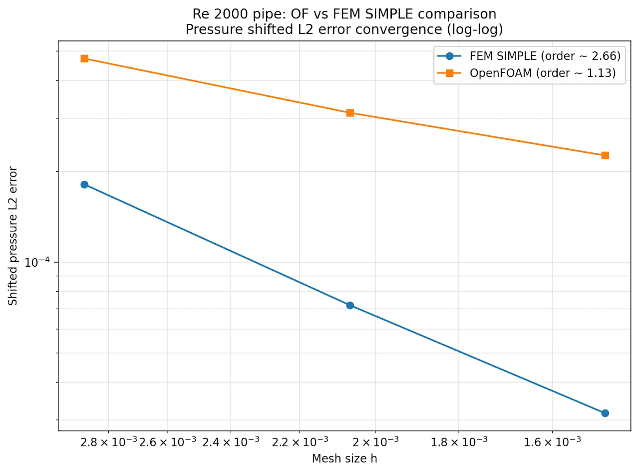
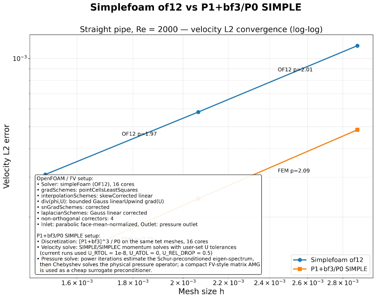
Straight-pipe tests were encouraging. In laminar Hagen-Poiseuille flow, including cases around Reynolds numbers 20 and 2000, the solver produced the expected pressure-gradient and velocity-profile convergence and compared well with a finite-volume SIMPLE reference. Those tests were important because they separated the basic mixed discretization and SIMPLE coupling from turbulence-model complications.

Figure 3: NodalS: Outer iterations for convergence vs OpenFOAM

Figure 4: NodalS wall time for convergence vs OpenFOAM

Figure 5: Pressure error comparison vs OpenFOAM

Figure 6: Velocity error vs OpenFOAM (alongwith scheme descriptions)

For the next step towards turbulent flow we aimed to produce our values for the VMFL003 Ansys benchmark. This benchmark uses a pipe that 500 diameters long and it exposed a geometric weakness rather than a fundamental algebraic one. Trying to represent its wall layer with tetrahedra while keeping the overall cell count manageable required strongly stretched elements. In that mesh family the tetrahedral formulation developed sliver-like cells and the turbulent pressure-drop error rose to roughly nine percent.

Figure 7: The tet mesh used for turbulent flow computations (mid plane cross section of the pipe geometry)

That result motivated a change of element shape rather than a change of the basic solver idea: preserve cellwise discontinuous pressure and shared face velocity enrichment, but move to hexahedra whose long axial aspect ratios remain much better conditioned.

5. Hex analogue: Q1+BF2/Q0

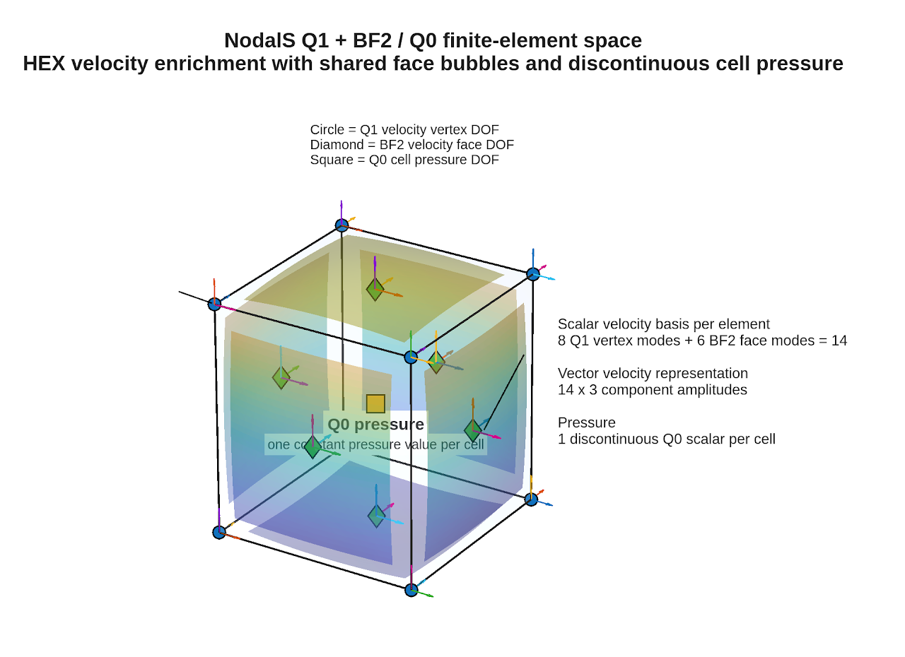
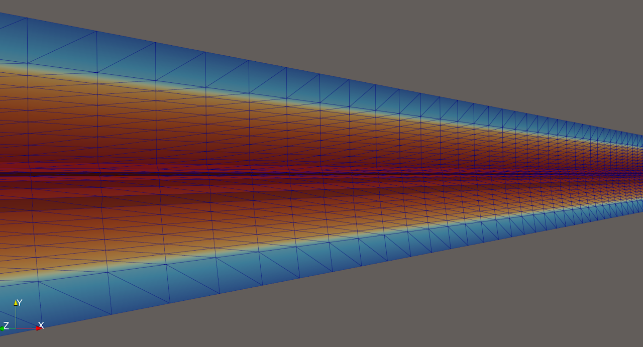
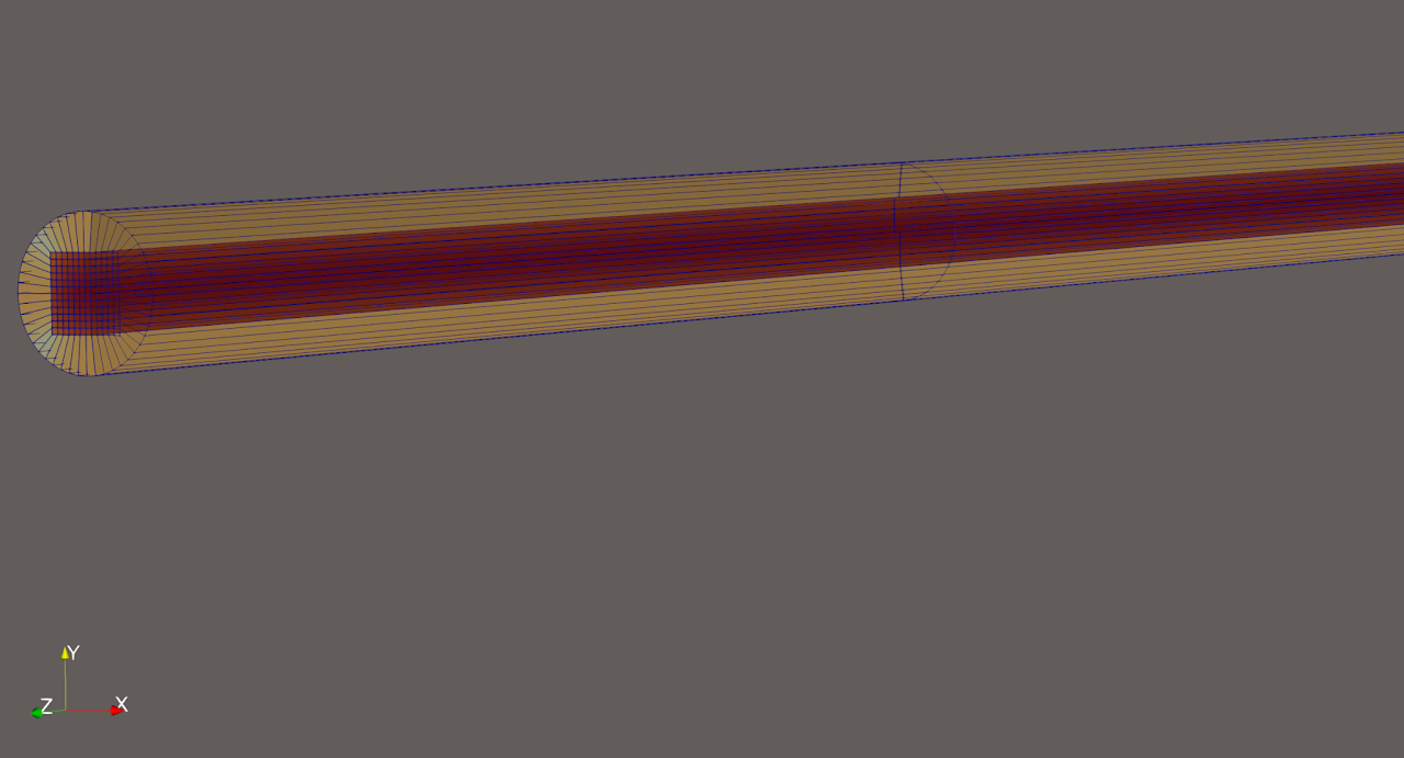
The strict-hex version of NodalS uses eight standard trilinear Q1 vertex modes plus six shared quadrilateral-face bubble modes per element. Each scalar velocity component therefore has 14 local modes, while pressure remains one discontinuous Q0 value per hex cell. (see figure 3)

Strict-hex mixed element used for the turbulent-pipe work

The intent is directly analogous to the tetrahedral element: the Q1 part provides the continuous low-order velocity field and the six face modes supply the additional flux-carrying directions needed by the mixed pressure coupling. The bubbles are shared face entities, not independent interior bubbles duplicated by each neighbouring cell.

Figure 8: The hex mesh used for turbulent flow computations (mid plane cut section)

The VMFL003 article mesh is deliberately coarse: an O-grid with 192 hexahedra in each cross-section and only 68 axial layers, for 13,056 cells in a 500D pipe. The first 20D uses 20 layers of length 1D, followed by 48 long layers of 10D. This is exactly the kind of geometry for which elongated, aligned hexes are appealing.

6. Cheap momentum smoothing with Chebyshev-Jacobi

A diagonal preconditioner is attractive for memory and parallelism, but plain Jacobi can be a poor smoother when the momentum operator becomes strongly anisotropic or badly scaled. The NodalS hex branch therefore uses higher-degree Chebyshev smoothing on top of Jacobi in PETSc's multigrid hierarchy.

Conceptual Chebyshev-accelerated Jacobi iteration

The practical advantage is that Chebyshev iteration needs only repeated sparse operator applications and diagonal scaling once useful spectral bounds are available. PETSc can estimate the relevant eigenvalue range and then apply a polynomial that damps the unwanted part of the spectrum more effectively than one Jacobi step.

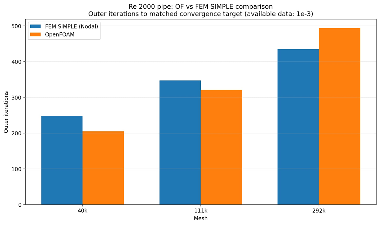
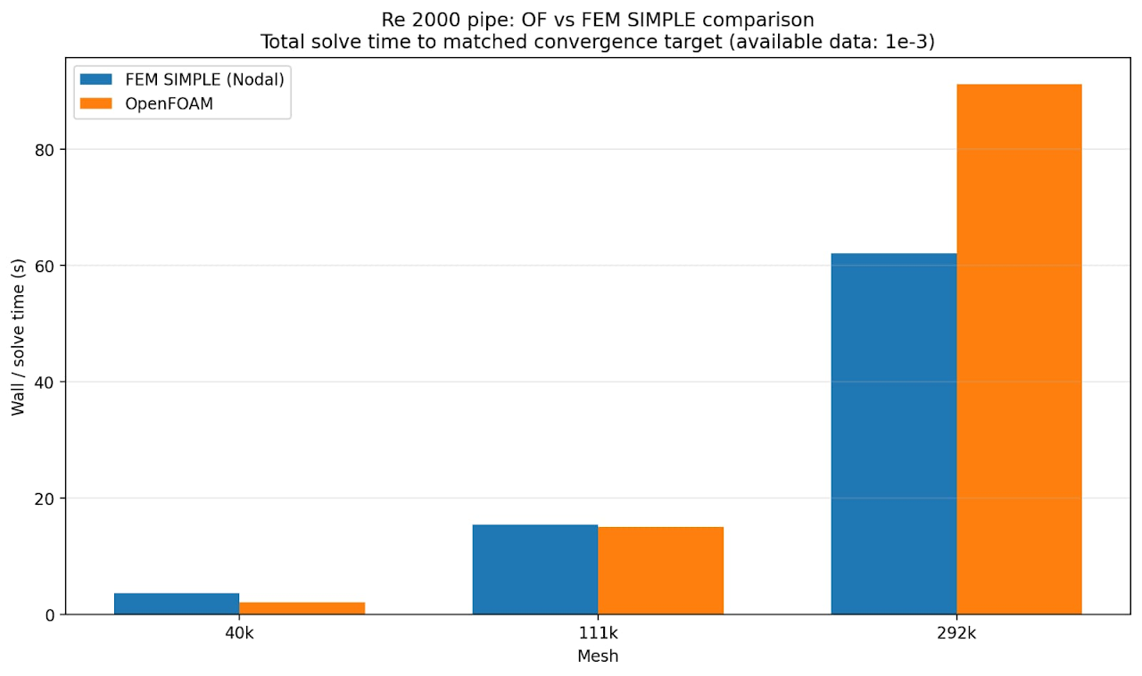
This became especially interesting in the turbulent runs. Plug, parabolic, and one-seventh-power-law inlet profiles could initially produce a difficult pressure/momentum transient with high Krylov iteration counts. Once the nonlinear state passed the steep entrance/start-up phase, the linear solves became much easier and the overall SIMPLE iteration converged. Interestingly for some cases this multigrid configuration led to much less iteration of the outer conjugate gradient than the conjugate gradient in OpenFOAM which was preconditioned with a gauss siedel based OpenFOAM GAMG.

However, this is a problem-specific observation, not a general robustness claim. The VMFL003 geometry is strongly aligned and the present wall model is specialized to a straight circular pipe. Still, the experiment is a positive sign for low-memory FE pressure-correction solvers built around sparse operator applications on a GPU.

7. Mixing length model

The turbulent-pipe solver was kept deliberately straightforward and simple for this elementary turbulence verification. This branch does not solve k, epsilon, omega, or any other transported turbulence variable. It uses a Nikuradse mixing-length closure evaluated at the volume quadrature points from the current velocity field.

Nikuradse pipe mixing length and algebraic eddy viscosity

The turbulent viscosity is therefore an algebraic consequence of the lagged SIMPLE velocity gradient. The accepted implementation updates the turbulent diffusion incrementally from one SIMPLE state to the next rather than storing a second full momentum matrix or a persistent cell-by-quadrature turbulent-viscosity field.

The calculation is initialized from a plug velocity. Because an exact plug has almost no interior strain, the initial volume eddy viscosity is nearly zero. The wall treatment supplies shear first; the velocity profile then develops, nonzero strain appears, and the algebraic turbulent viscosity emerges naturally in subsequent SIMPLE iterations.

8. A weak Spalding wall treatment

The wall model was one of the most important parts of the development.

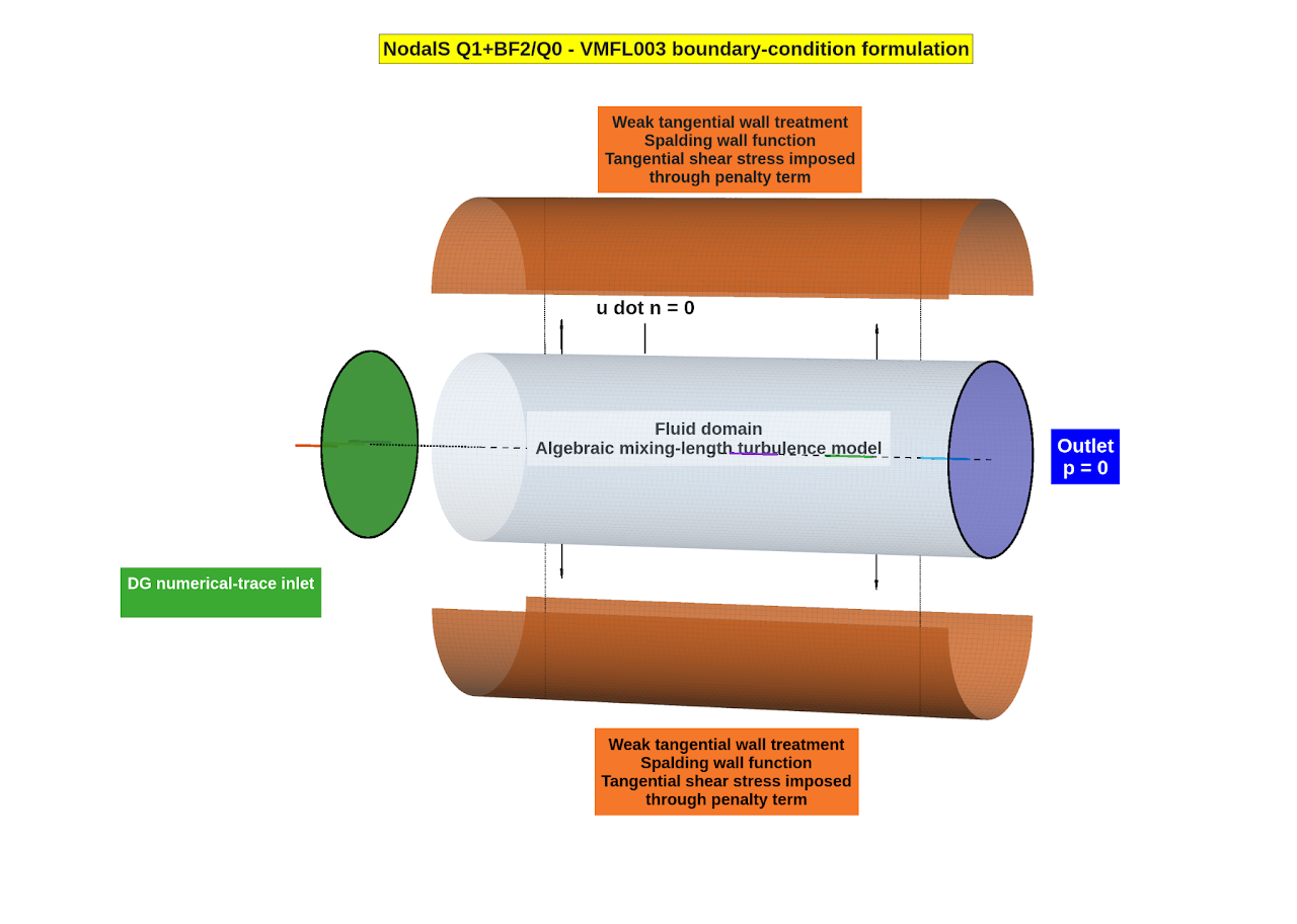
The accepted hex implementation evaluates the full Q1+BF2 velocity at a geometrically defined off-wall point. For each wall quadrature point it moves inward to the wall-adjacent element's reference midplane, maps both points to physical space, computes the true radial wall-normal distance, and inverts the Spalding relation for friction velocity.

Spalding relation used to obtain friction velocity and the weak wall coefficient

The resulting coefficient acts as a weak streamwise wall traction. For this straight z-aligned pipe, the two cross-stream velocity components are strongly clamped while the axial component is left free to respond to the wall model. This should therefore be described as a pipe-specific weak tangential wall treatment, not yet as a generic arbitrary-wall implementation.

An additional molecular Nitsche-consistency contribution was tested but eventually disabled in the accepted benchmark configuration because it duplicated part of the drag already represented by the Spalding traction. The final article case therefore uses the Spalding-derived wall traction without that extra molecular wall term.

9. The inlet-rim problem and the DG numerical trace

A strong plug inlet creates a subtle incompatibility at the circular rim: the same globally continuous velocity entities are asked to satisfy both the inlet plug and the wall condition. The early strong-CG inlet could force the face modes to repair flux near the wall and produced a large artificial entrance pressure spike that did not disappear when the nonlinear tolerance was tightened.

The accepted solution was to keep the volume method continuous but impose the inlet as a DG-style numerical trace. The inlet Q1 and BF2 volume unknowns remain free; the prescribed external trace supplies the mass flux and the inflow state.

Prescribed inlet trace used in the cellwise continuity operator

For first-layer cells, the Q0 continuity equation therefore uses the prescribed inlet flux rather than the finite-element volume trace. This fixes the total inlet mass flow exactly in the discrete continuity equation.

Convection receives a physical inflow/upwind correction using the prescribed trace, while viscous diffusion at the inlet is handled with a penalty-free nonsymmetric Nitsche term. This localized DG boundary idea removed most of the artificial entrance loss while leaving the rest of the velocity space continuous.

Figure 9: Custom mixed finite-element SIMPLE solver - NodalS

Figure 10: The DG inlet ensures a smooth inlet progression and avoids the entrance loss

10. VMFL003: results

The ANSYS VMFL003 verification problem is turbulent pressure drop through a straight circular pipe. The geometry used here has D = 0.004 m and L = 2 m = 500D, with bulk speed 50 m/s, density 1.225 kg/m3 and dynamic viscosity 1.7894e-5 kg/(m s). The corresponding Reynolds number is about 13,692. The official benchmark pressure drop is 21,744 Pa.

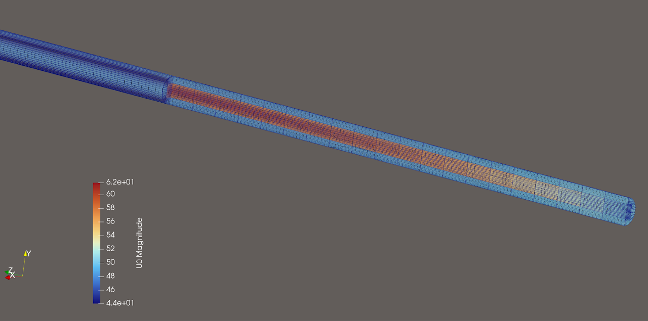
The primary NodalS article run uses the 13,056-cell strict-hex O-grid described above, SIMPLEC, the Nikuradse algebraic mixing length, the corrected off-wall Spalding treatment, and the DG numerical inlet trace. Its representative wall resolution is approximately y+ = 29.

Darcy friction factor used for the developed-flow comparisons

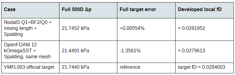
The eye-catching NodalS full-length result is 21,745.20 Pa, only about +0.0055% from the official 21,744 Pa target. However, this is due to a fortuitous cancellation with the positive inlet error during the flow profile development. A more accurate number the friction factor error in the developed region, roughly 50D to 450D. Here, the NodalS Darcy friction factor was about 0.028195, approximately 0.93% below the smooth Moody/Colebrook value used for the local comparison.

The reason is visible when the pipe is divided into axial zones. The first 50D carries a larger developing/entrance loss, while the long developed portion is slightly under the smooth-pipe friction reference. Over the complete 500D length the two effects almost cancel.

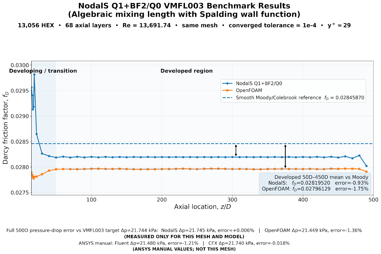
Figure 11: Results of the VMFL003 benchmark for the specific mesh (section 5)

On the same 13,056-cell mesh, the OpenFOAM 12 comparison used k-omega SST with Spalding-type turbulence wall functions and a strong fixedValue plug inlet. Its full pressure drop was about 21.449 kPa, or -1.36% from the VMFL003 target, and its developed local friction was about 1.75% below the same smooth Moody/Colebrook reference.

This should be read as a same-mesh solver/model comparison, not as a pure discretization comparison. NodalS uses a zero-equation algebraic mixing-length closure and a weak wall traction; OpenFOAM uses transported SST variables, strong no-slip velocity, and its own wall-function machinery.

11. What happened when y+ was changed?

An increase in the y+ in the range of 60-100 through a mesh change resulted in a similar result of ~1% error of friction factor for the developed profile. At lower y+ however, the model failure was evident. At lower y+ most meshes did not converge due to high aspect ratio of the hex. Instead the same aspect ratio from the earlier mesh (section 5) was maintained and a 96,768-cell 100D graded mesh was created. This mesh moved the near-wall sampling into roughly y+ = 9-27, with a mean around 17. The nonlinear solution still converged and the downstream friction zones became essentially flat, but the developed Darcy friction rose to about 0.03308: roughly +16.5% relative to the VMFL003 target friction. We were still unable to get OpenFOAM to converge on this mesh even with powerful pressure solver settings.

That behaviour is physically consistent with the limitations of the closure. Near the wall, an undamped Prandtl/Nikuradse mixing length behaves like a log-layer model. Spalding gives a composite relation between mean velocity and wall shear, but it does not automatically correct the separate volume model νt = l²|S| inside the buffer layer.

Further steps for making the model more robust to low y+ would introduce a near-wall damping mechanism such as van Driest damping, or to move to a more complete algebraic model such as Baldwin-Lomax, while keeping the already-tested Q1+BF2/Q0 pressure-velocity architecture unchanged.

12. What this experiment says - and what it does not

A discontinuous constant pressure space can give one integrated continuity equation per cell creating a beneficial cell wise mass conservation
Shared face-enrichment can make a low-order mixed FE pair pressure-stable without adding PSPG or Rhie-Chow pressure dissipation.
That topology is compatible with a SIMPLE/SIMPLEC pressure correction based on a cheap diagonal approximation to the momentum inverse.
The tetrahedral idea transfers naturally to a Q1+BF2/Q0 hexahedral analogue, which is attractive for very long aligned domains.
Chebyshev-accelerated Jacobi can be a useful low-memory smoother for the tested turbulent pipe, although this is not a universal robustness result.
A simple algebraic mixing-length closure can give good log-layer results on this benchmark, but it is not a low-y+ turbulence model without additional damping.

The strongest result is therefore not the almost exact full-pipe pressure-drop number by itself. The more interesting result is architectural: a custom mixed finite-element discretization with discontinuous cell pressure and face-enriched continuous velocity can be organized into a familiar segregated SIMPLE workflow, with compact pressure preconditioning and sparse, GPU-friendly linear algebra.

For NodalS, the next interesting questions are broader geometry support, a generic tangential wall formulation, near-wall-damped algebraic turbulence, and eventually transported turbulence and heat-transfer equations. Those extensions can be added without abandoning the central pressure-velocity arrangement.

References and benchmark notes

P. E. Farrell, L. Mitchell and F. Wechsung, “An Augmented Lagrangian Preconditioner for the 3D Stationary Incompressible Navier-Stokes Equations at High Reynolds Number,” arXiv:1810.03315, 2019. The paper discusses the [P1 ⊕ B3^F]^3-P0 face-bubble-enriched pair used as the starting point for the tetrahedral NodalS formulation.
ANSYS Fluid Dynamics Verification Manual, VMFL003: Pressure Drop in Turbulent Flow Through a Pipe. Official target pressure drop used here: 21,744 Pa.
NodalS VMFL003 turbulence benchmark handoff, 3 September 2026. Numerical values, mesh definition, accepted boundary-condition semantics, and low-y+ diagnostics in this article follow the archived benchmark state.

Note on the published comparison: the ANSYS manual Fluent/CFX values use the manual's own model and meshes and are not same-mesh NodalS results. The OpenFOAM comparison described above is the same 13,056-hex topology, but it uses a different turbulence closure and different wall-boundary formulation.