<?xml version="1.0" encoding="utf-8"?>
<feed xmlns="http://www.w3.org/2005/Atom" xmlns:media="http://search.yahoo.com/mrss/">
    <title>Mathbridge</title>
    <link href="https://jade-speculoos-11a861.netlify.app/feed.xml" rel="self" />
    <link href="https://jade-speculoos-11a861.netlify.app" />
    <updated>2026-09-17T15:39:56+05:30</updated>
    <author>
        <name>Shubhankar</name>
    </author>
    <id>https://jade-speculoos-11a861.netlify.app</id>

    <entry>
        <title>Custom mixed finite-element SIMPLE solver</title>
        <author>
            <name>Dr. Jaydeep Deshpande</name>
        </author>
        <link href="https://jade-speculoos-11a861.netlify.app/custom-mixed-finite-element-simple-solver.html"/>
        <id>https://jade-speculoos-11a861.netlify.app/custom-mixed-finite-element-simple-solver.html</id>

        <updated>2026-09-10T14:37:00+05:30</updated>
            <summary type="html">
                <![CDATA[
                    Numerical experiments on Face enriched P1/P0 or Q1/Q0 FEM function space For incompressible flow, the familiar numerical tension is between velocity-pressure stability, local mass balance, robustness at high Reynolds number, and cost. A collocated finite-volume method is attractive because both the velocity and pressure unknowns&hellip;
                ]]>
            </summary>
        <content type="html">
            <![CDATA[
                <section id="h.48b84d2315451c26_16" class="yaqOZd">
<div class="mYVXT">
<div class="LS81yb VICjCf j5pSsc db35Fc" tabindex="-1">
<div class="hJDwNd-AhqUyc-uQSCkd Ft7HRd-AhqUyc-uQSCkd purZT-AhqUyc-II5mzb ZcASvf-AhqUyc-II5mzb pSzOP-AhqUyc-qWD73c Ktthjf-AhqUyc-qWD73c JNdkSc SQVYQc">
<div class="JNdkSc-SmKAyb LkDMRd">
<div class="">
<div class="oKdM2c ZZyype Kzv0Me">
<div id="h.48b84d2315451c26_13" class="hJDwNd-AhqUyc-uQSCkd Ft7HRd-AhqUyc-uQSCkd jXK9ad D2fZ2 zu5uec OjCsFc dmUFtb wHaque g5GTcb">
<div class="jXK9ad-SmKAyb">
<div class="tyJCtd mGzaTb Depvyb baZpAe">
<p class="zfr3Q CDt4Ke  align-center" dir="ltr"><em><span class="C9DxTc ">Numerical experiments on Face enriched P1/P0 or Q1/Q0 FEM function space</span></em></p>
<p dir="ltr"> </p>
</div>
</div>
</div>
</div>
</div>
</div>
</div>
</div>
</div>
</section>
<section id="h.41d9d1b547f2c30b_33" class="yaqOZd">
<div class="mYVXT">
<div class="LS81yb VICjCf j5pSsc db35Fc" tabindex="-1">
<div class="hJDwNd-AhqUyc-uQSCkd Ft7HRd-AhqUyc-uQSCkd purZT-AhqUyc-II5mzb ZcASvf-AhqUyc-II5mzb pSzOP-AhqUyc-qWD73c Ktthjf-AhqUyc-qWD73c JNdkSc SQVYQc">
<div class="JNdkSc-SmKAyb LkDMRd">
<div class="">
<div class="oKdM2c ZZyype Kzv0Me">
<div id="h.41d9d1b547f2c30b_30" class="hJDwNd-AhqUyc-uQSCkd Ft7HRd-AhqUyc-uQSCkd jXK9ad D2fZ2 zu5uec OjCsFc dmUFtb wHaque g5GTcb">
<div class="jXK9ad-SmKAyb">
<div class="tyJCtd mGzaTb Depvyb baZpAe"><small class="zfr3Q TMjjoe CDt4Ke " dir="ltr"><span class="C9DxTc ">The article describes a SIMPLE-type incompressible-flow solver built with mixed finite elements discretization. The central idea is to use a continuous velocity space enriched by shared face degrees of freedom, pair it with one discontinuous pressure unknown per cell, and exploit that topology to build a cheap pressure-correction operator. </span></small><small class="zfr3Q TMjjoe CDt4Ke " dir="ltr"><span class="C9DxTc ">The objective was to document a useful numerical experiment, in which a mixed FE formulation can retain a local cellwise continuity equation, avoid pressure-stabilization devices such as PSPG or Rhie-Chow interpolation, and still admit a very cheap SIMPLE-like pressure correction.</span></small></div>
</div>
</div>
</div>
</div>
</div>
</div>
</div>
</div>
</section>
<section id="h.48b84d2315451c26_24" class="yaqOZd">
<div class="mYVXT">
<div class="LS81yb VICjCf j5pSsc db35Fc" tabindex="-1">
<div class="hJDwNd-AhqUyc-uQSCkd Ft7HRd-AhqUyc-uQSCkd purZT-AhqUyc-II5mzb ZcASvf-AhqUyc-II5mzb pSzOP-AhqUyc-qWD73c Ktthjf-AhqUyc-qWD73c JNdkSc SQVYQc">
<div class="JNdkSc-SmKAyb LkDMRd">
<div class="">
<div class="oKdM2c ZZyype Kzv0Me">
<div id="h.48b84d2315451c26_21" class="hJDwNd-AhqUyc-uQSCkd Ft7HRd-AhqUyc-uQSCkd jXK9ad D2fZ2 zu5uec OjCsFc dmUFtb wHaque g5GTcb">
<div class="jXK9ad-SmKAyb">
<div class="tyJCtd mGzaTb Depvyb baZpAe">
<h2 class="CjVfdc"><span class="C9DxTc ">1. Why a mixed finite-element SIMPLE solver?</span></h2>
<h3 id="h.i7tnn0n3tdbz_l" class="zfr3Q OmQG5e CDt4Ke " dir="ltr"></h3>
<p class="zfr3Q CDt4Ke " dir="ltr"><span class="C9DxTc ">For incompressible flow, the familiar numerical tension is between velocity-pressure stability, local mass balance, robustness at high Reynolds number, and cost. A collocated finite-volume method is attractive because both the velocity and pressure unknowns are cell-centred. A collocated formulation much like equal order finite element pairs, runs into the inf-sup problem: in short the pressure -velocity discretization is rank deficient and thus its pressure to velocity relationship is not adequately represented. The problem is circumvented through the addition of dissipation terms like Rhie-Chow interpolation, Brezzi-Pitkaranta term or pressure stabilized Petrov-Galerkin (PSPG) term to the pressure-pressure block of incompressible Navier-Stokes. Staggered FV discretizations which treat pressure at the cell center and velocity as constant flux face variables naturally avoid the rank-deficiency and are able to provide a formulation that conserves mass accurately. However, an ‘unstructured FV staggering’ is still not a solved problem. What even does staggering mean in an unstructured sense? In this respect finite-elements provide a cleaner approach with mixed elements like P2-P1 (quadratic velocity, linear pressure) which can be used on unstructured meshes without the rank deficiency. However these implementations are typically implemented in FEM softwares in continuous galerkin format, which does not provide local mass balance since the pressure test function is continuous. As against this discontinuous P2-P1 formulations provide the local mass balance but are extremely heavy to run. The majority of FEM literature though is quite focused on monolithic solvers which do not solve Navier Stokes in segregated manner. This results in even matrix free FEM solvers reaching memory requirements close to 15-20 GB/ million cells. Such a big memory bandwidth creates a slow solver. A straightforward solution could be to use a low-order continuous finite-element pair continuous linear (P1) velocity with discontinuous zeroth order (P0) pressure. Unfortunately, though this function space is mixed, it is not inf-sup stable.</span></p>
<p class="zfr3Q CDt4Ke " dir="ltr"><span class="C9DxTc ">We thus started from a third option derived originally by Farrell et al (2019) for the Augmented Lagrangian Preconditioner.</span></p>
</div>
</div>
</div>
</div>
</div>
</div>
</div>
</div>
</div>
</section>
<section id="h.48b84d2315451c26_48" class="yaqOZd">
<div class="mYVXT">
<div class="LS81yb VICjCf j5pSsc db35Fc" tabindex="-1">
<div class="hJDwNd-AhqUyc-OiUrBf Ft7HRd-AhqUyc-OiUrBf purZT-AhqUyc-II5mzb ZcASvf-AhqUyc-II5mzb pSzOP-AhqUyc-qWD73c Ktthjf-AhqUyc-qWD73c JNdkSc SQVYQc yYI8W HQwdzb">
<div class="JNdkSc-SmKAyb LkDMRd">
<div class="">
<div class="oKdM2c ZZyype Kzv0Me">
<div id="h.41d9d1b547f2c30b_34" class="hJDwNd-AhqUyc-OiUrBf Ft7HRd-AhqUyc-OiUrBf jXK9ad D2fZ2 zu5uec OjCsFc dmUFtb">
<div class="jXK9ad-SmKAyb">
<div class="tyJCtd baZpAe">
<div class="t3iYD">
<figure class="post__image"><img loading="lazy" role="img" src="https://jade-speculoos-11a861.netlify.app/media/posts/6/1.png" alt="Figure 1: The P1+BF3/P0 function space" width="1280" height="867" sizes="(max-width: 1920px) 100vw, 1920px" srcset="https://jade-speculoos-11a861.netlify.app/media/posts/6/responsive/1-xs.png 640w ,https://jade-speculoos-11a861.netlify.app/media/posts/6/responsive/1-sm.png 768w ,https://jade-speculoos-11a861.netlify.app/media/posts/6/responsive/1-md.png 1024w ,https://jade-speculoos-11a861.netlify.app/media/posts/6/responsive/1-lg.png 1366w ,https://jade-speculoos-11a861.netlify.app/media/posts/6/responsive/1-xl.png 1600w ,https://jade-speculoos-11a861.netlify.app/media/posts/6/responsive/1-2xl.png 1920w">
<figcaption><span class="C9DxTc ">Figure 1: The P1+BF3/P0 function space</span></figcaption>
</figure>
</div>
</div>
</div>
</div>
</div>
</div>
</div>
</div>
</div>
</div>
</section>
<section id="h.48b84d2315451c26_54" class="yaqOZd">
<div class="mYVXT">
<div class="LS81yb VICjCf j5pSsc db35Fc" tabindex="-1">
<div class="hJDwNd-AhqUyc-uQSCkd Ft7HRd-AhqUyc-uQSCkd purZT-AhqUyc-II5mzb ZcASvf-AhqUyc-II5mzb pSzOP-AhqUyc-qWD73c Ktthjf-AhqUyc-qWD73c JNdkSc SQVYQc">
<div class="JNdkSc-SmKAyb LkDMRd">
<div class="">
<div class="oKdM2c ZZyype Kzv0Me">
<div id="h.48b84d2315451c26_51" class="hJDwNd-AhqUyc-uQSCkd Ft7HRd-AhqUyc-uQSCkd jXK9ad D2fZ2 zu5uec OjCsFc dmUFtb wHaque g5GTcb">
<div class="jXK9ad-SmKAyb">
<div class="tyJCtd mGzaTb Depvyb baZpAe">
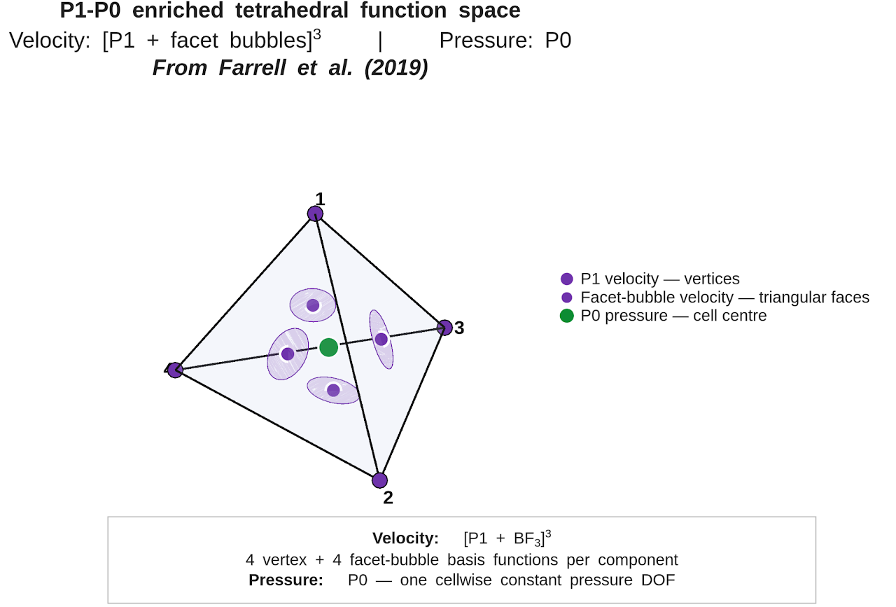
<p class="zfr3Q CDt4Ke " dir="ltr"><span class="C9DxTc ">The velocity remains globally continuous, but it is enriched with velocity degrees of freedom associated with element faces. The pressure is discontinuous and constant within each cell, which allows the pressure test function to test local mass balance (see the next section). Additionally the topology appears surprisingly close to a staggered method: pressure lives in cells, while the additional shared velocity modes help in providing the discrete divergence that couples with neighbouring cells without adding an artificial pressure-dissipation term.</span></p>
</div>
</div>
</div>
</div>
</div>
</div>
</div>
</div>
</div>
</section>
<section id="h.48b84d2315451c26_58" class="yaqOZd">
<div class="mYVXT">
<div class="LS81yb VICjCf j5pSsc db35Fc" tabindex="-1">
<div class="hJDwNd-AhqUyc-OiUrBf Ft7HRd-AhqUyc-OiUrBf purZT-AhqUyc-II5mzb ZcASvf-AhqUyc-II5mzb pSzOP-AhqUyc-qWD73c Ktthjf-AhqUyc-qWD73c JNdkSc SQVYQc yYI8W HQwdzb">
<div class="JNdkSc-SmKAyb LkDMRd">
<div class="">
<div class="oKdM2c ZZyype Kzv0Me">
<div id="h.48b84d2315451c26_55" class="hJDwNd-AhqUyc-OiUrBf Ft7HRd-AhqUyc-OiUrBf jXK9ad D2fZ2 zu5uec OjCsFc dmUFtb">
<div class="jXK9ad-SmKAyb">
<div class="tyJCtd baZpAe">
<div class="t3iYD">
<figure class="post__image"><figure class="post__image"><img loading="lazy"  src="https://jade-speculoos-11a861.netlify.app/media/posts/6/2.png" alt="Governing incompressible momentum and continuity equations" width="1280" height="218" sizes="(max-width: 1920px) 100vw, 1920px" srcset="https://jade-speculoos-11a861.netlify.app/media/posts/6/responsive/2-xs.png 640w ,https://jade-speculoos-11a861.netlify.app/media/posts/6/responsive/2-sm.png 768w ,https://jade-speculoos-11a861.netlify.app/media/posts/6/responsive/2-md.png 1024w ,https://jade-speculoos-11a861.netlify.app/media/posts/6/responsive/2-lg.png 1366w ,https://jade-speculoos-11a861.netlify.app/media/posts/6/responsive/2-xl.png 1600w ,https://jade-speculoos-11a861.netlify.app/media/posts/6/responsive/2-2xl.png 1920w"></figure>
<figcaption><span class="C9DxTc ">Governing incompressible momentum and continuity equations</span></figcaption>
</figure>
</div>
</div>
</div>
</div>
</div>
</div>
</div>
</div>
<div class="hJDwNd-AhqUyc-ibL1re Ft7HRd-AhqUyc-ibL1re JNdkSc SQVYQc L6cTce-purZT L6cTce-pSzOP">
<div class="JNdkSc-SmKAyb LkDMRd">
<div class=""><span style="font-size: inherit;">Convection can be treated centrally, or streamline-upwind/Petrov-Galerkin stabilization can be added when desired. Crucially, upwinding acts through the momentum discretization; pressure is not stabilized by a PSPG term, and the solver does not need a Rhie-Chow-style pressure filter.</span></div>
</div>
</div>
</div>
</div>
</section>
<section id="h.48b84d2315451c26_62" class="yaqOZd">
<div class="mYVXT">
<div class="LS81yb VICjCf j5pSsc db35Fc" tabindex="-1">
<div class="hJDwNd-AhqUyc-uQSCkd Ft7HRd-AhqUyc-uQSCkd purZT-AhqUyc-II5mzb ZcASvf-AhqUyc-II5mzb pSzOP-AhqUyc-qWD73c Ktthjf-AhqUyc-qWD73c JNdkSc SQVYQc">
<div class="JNdkSc-SmKAyb LkDMRd">
<div class="">
<div class="oKdM2c ZZyype Kzv0Me">
<div id="h.48b84d2315451c26_59" class="hJDwNd-AhqUyc-uQSCkd Ft7HRd-AhqUyc-uQSCkd jXK9ad D2fZ2 zu5uec OjCsFc dmUFtb wHaque g5GTcb">
<div class="jXK9ad-SmKAyb">
<div class="tyJCtd mGzaTb Depvyb baZpAe">
<p class="zfr3Q CDt4Ke " dir="ltr"><span class="C9DxTc ">Note that this tetrahedral element that motivated the original NodalS solver is the face-bubble-enriched pair discussed by Farrell, Mitchell and Wechsung in their 2019 high-Reynolds-number preconditioning work and is not the invention of the current author. More precisely, the formulation enriches all three components of P1 velocity with cubic facet bubbles and pairs the result with discontinuous P0 pressure.</span></p>
</div>
</div>
</div>
</div>
</div>
</div>
</div>
</div>
</div>
</section>
<section id="h.48b84d2315451c26_66" class="yaqOZd">
<div class="mYVXT">
<div class="LS81yb VICjCf j5pSsc db35Fc" tabindex="-1">
<div class="hJDwNd-AhqUyc-OiUrBf Ft7HRd-AhqUyc-OiUrBf purZT-AhqUyc-II5mzb ZcASvf-AhqUyc-II5mzb pSzOP-AhqUyc-qWD73c Ktthjf-AhqUyc-qWD73c JNdkSc SQVYQc yYI8W HQwdzb">
<div class="JNdkSc-SmKAyb LkDMRd">
<div class="">
<div class="oKdM2c ZZyype Kzv0Me">
<div id="h.48b84d2315451c26_63" class="hJDwNd-AhqUyc-OiUrBf Ft7HRd-AhqUyc-OiUrBf jXK9ad D2fZ2 zu5uec OjCsFc dmUFtb">
<div class="jXK9ad-SmKAyb">
<div class="tyJCtd baZpAe">
<div class="t3iYD">
<figure class="post__image"><img loading="lazy" role="img" src="https://jade-speculoos-11a861.netlify.app/media/posts/6/3.png" alt="" width="1280" height="161" sizes="(max-width: 1920px) 100vw, 1920px" srcset="https://jade-speculoos-11a861.netlify.app/media/posts/6/responsive/3-xs.png 640w ,https://jade-speculoos-11a861.netlify.app/media/posts/6/responsive/3-sm.png 768w ,https://jade-speculoos-11a861.netlify.app/media/posts/6/responsive/3-md.png 1024w ,https://jade-speculoos-11a861.netlify.app/media/posts/6/responsive/3-lg.png 1366w ,https://jade-speculoos-11a861.netlify.app/media/posts/6/responsive/3-xl.png 1600w ,https://jade-speculoos-11a861.netlify.app/media/posts/6/responsive/3-2xl.png 1920w">
<figcaption>Original tetrahedral NodalS velocity-pressure pair</figcaption>
</figure>
</div>
</div>
</div>
</div>
</div>
<div class="oKdM2c ZZyype">
<div id="h.48b84d2315451c26_69" class="hJDwNd-AhqUyc-OiUrBf Ft7HRd-AhqUyc-OiUrBf jXK9ad D2fZ2 zu5uec wHaque g5GTcb">
<div class="jXK9ad-SmKAyb">
<div class="tyJCtd mGzaTb Depvyb baZpAe"><span style="font-size: inherit;">The face bubble is just an extra shared velocity degree of freedom attached to a face and is able to participate int typical FEM continuous galerkin assembly. However note that its contribution goes to zero at the other face nodes, thus it provides an added a degree of independence to the solver for attacking the face contributions that are shared exactly between 2 cells, unlike the nodes which are shared with a large number of neighboring cells. This feature is also later preserved in the hexahedral analogue.</span></div>
</div>
</div>
</div>
</div>
</div>
</div>
</div>
</div>
</section>
<section id="h.48b84d2315451c26_86" class="yaqOZd">
<div class="mYVXT">
<div class="LS81yb VICjCf j5pSsc db35Fc" tabindex="-1">
<div class="hJDwNd-AhqUyc-OiUrBf Ft7HRd-AhqUyc-OiUrBf purZT-AhqUyc-II5mzb ZcASvf-AhqUyc-II5mzb pSzOP-AhqUyc-qWD73c Ktthjf-AhqUyc-qWD73c JNdkSc SQVYQc yYI8W HQwdzb">
<div class="JNdkSc-SmKAyb LkDMRd">
<div class="">
<div class="oKdM2c ZZyype Kzv0Me">
<div id="h.48b84d2315451c26_83" class="hJDwNd-AhqUyc-OiUrBf Ft7HRd-AhqUyc-OiUrBf jXK9ad D2fZ2 zu5uec OjCsFc dmUFtb">
<div class="jXK9ad-SmKAyb">
<div class="tyJCtd baZpAe">
<div class="t3iYD">
<figure class="CENy8b post__image"><img loading="lazy" role="img" src="https://jade-speculoos-11a861.netlify.app/media/posts/6/4.png" alt="Figure 2: The Q1+BF2/Q0 function space" width="1280" height="930" sizes="(max-width: 1920px) 100vw, 1920px" srcset="https://jade-speculoos-11a861.netlify.app/media/posts/6/responsive/4-xs.png 640w ,https://jade-speculoos-11a861.netlify.app/media/posts/6/responsive/4-sm.png 768w ,https://jade-speculoos-11a861.netlify.app/media/posts/6/responsive/4-md.png 1024w ,https://jade-speculoos-11a861.netlify.app/media/posts/6/responsive/4-lg.png 1366w ,https://jade-speculoos-11a861.netlify.app/media/posts/6/responsive/4-xl.png 1600w ,https://jade-speculoos-11a861.netlify.app/media/posts/6/responsive/4-2xl.png 1920w">
<figcaption><span class="C9DxTc ">Figure 2: The Q1+BF2/Q0 function space</span></figcaption>
</figure>
</div>
</div>
</div>
</div>
</div>
</div>
</div>
</div>
</div>
</div>
</section>
<section id="h.48b84d2315451c26_92" class="yaqOZd">
<div class="mYVXT">
<div class="LS81yb VICjCf j5pSsc db35Fc" tabindex="-1">
<div class="hJDwNd-AhqUyc-uQSCkd Ft7HRd-AhqUyc-uQSCkd purZT-AhqUyc-II5mzb ZcASvf-AhqUyc-II5mzb pSzOP-AhqUyc-qWD73c Ktthjf-AhqUyc-qWD73c JNdkSc SQVYQc">
<div class="JNdkSc-SmKAyb LkDMRd">
<div class="">
<div class="oKdM2c ZZyype Kzv0Me">
<div id="h.48b84d2315451c26_89" class="hJDwNd-AhqUyc-uQSCkd Ft7HRd-AhqUyc-uQSCkd jXK9ad D2fZ2 zu5uec OjCsFc dmUFtb wHaque g5GTcb">
<div class="jXK9ad-SmKAyb">
<div class="tyJCtd mGzaTb Depvyb baZpAe">
<h2 class="CjVfdc"><span class="C9DxTc ">2. Why discontinuous cell pressure is useful</span></h2>
<h3 id="h.dkvzqlb2ap83_l" class="zfr3Q OmQG5e CDt4Ke " dir="ltr"></h3>
<p class="zfr3Q CDt4Ke " dir="ltr"><span class="C9DxTc ">The pressure space contains one constant test function per cell. Since pressure acts like the lagrange multiplier enforcing the continuity/mass balance, the pressure test function is utilized on the continuity equation assembly. This has an immediate consequence for continuity: choosing the pressure test function to be one on a particular element and zero elsewhere enforces the integrated divergence equation on that element in a manner which closer to how traditional FVM does.</span></p>
</div>
</div>
</div>
</div>
</div>
</div>
</div>
</div>
</div>
</section>
<section id="h.48b84d2315451c26_96" class="yaqOZd">
<div class="mYVXT">
<div class="LS81yb VICjCf j5pSsc db35Fc" tabindex="-1">
<div class="hJDwNd-AhqUyc-OiUrBf Ft7HRd-AhqUyc-OiUrBf purZT-AhqUyc-II5mzb ZcASvf-AhqUyc-II5mzb pSzOP-AhqUyc-qWD73c Ktthjf-AhqUyc-qWD73c JNdkSc SQVYQc yYI8W HQwdzb">
<div class="JNdkSc-SmKAyb LkDMRd">
<div class="">
<div class="oKdM2c ZZyype Kzv0Me">
<div id="h.48b84d2315451c26_93" class="hJDwNd-AhqUyc-OiUrBf Ft7HRd-AhqUyc-OiUrBf jXK9ad D2fZ2 zu5uec OjCsFc dmUFtb">
<div class="jXK9ad-SmKAyb">
<div class="tyJCtd baZpAe">
<div class="t3iYD">
<figure class="CENy8b post__image"><img loading="lazy" role="img" src="https://jade-speculoos-11a861.netlify.app/media/posts/6/5.png" alt="The Q0/P0 pressure equation is one integrated mass-balance equation per cell" width="1280" height="161" sizes="(max-width: 1920px) 100vw, 1920px" srcset="https://jade-speculoos-11a861.netlify.app/media/posts/6/responsive/5-xs.png 640w ,https://jade-speculoos-11a861.netlify.app/media/posts/6/responsive/5-sm.png 768w ,https://jade-speculoos-11a861.netlify.app/media/posts/6/responsive/5-md.png 1024w ,https://jade-speculoos-11a861.netlify.app/media/posts/6/responsive/5-lg.png 1366w ,https://jade-speculoos-11a861.netlify.app/media/posts/6/responsive/5-xl.png 1600w ,https://jade-speculoos-11a861.netlify.app/media/posts/6/responsive/5-2xl.png 1920w">
<figcaption><span class="C9DxTc ">The Q0/P0 pressure equation is one integrated mass-balance equation per cell</span></figcaption>
</figure>
</div>
</div>
</div>
</div>
</div>
</div>
</div>
</div>
</div>
</div>
</section>
<section id="h.48b84d2315451c26_102" class="yaqOZd">
<div class="mYVXT">
<div class="LS81yb VICjCf j5pSsc db35Fc" tabindex="-1">
<div class="hJDwNd-AhqUyc-uQSCkd Ft7HRd-AhqUyc-uQSCkd purZT-AhqUyc-II5mzb ZcASvf-AhqUyc-II5mzb pSzOP-AhqUyc-qWD73c Ktthjf-AhqUyc-qWD73c JNdkSc SQVYQc">
<div class="JNdkSc-SmKAyb LkDMRd">
<div class="">
<div class="oKdM2c ZZyype Kzv0Me">
<div id="h.48b84d2315451c26_99" class="hJDwNd-AhqUyc-uQSCkd Ft7HRd-AhqUyc-uQSCkd jXK9ad D2fZ2 zu5uec OjCsFc dmUFtb wHaque g5GTcb">
<div class="jXK9ad-SmKAyb">
<div class="tyJCtd mGzaTb Depvyb baZpAe">
<p class="zfr3Q CDt4Ke " dir="ltr"><span class="C9DxTc ">This is the sense in which the method is locally conservative. Note that it does not say that every pointwise or higher-order moment of divergence vanishes inside a cell. It says that the net flux through the cell boundary is zero to the accuracy of the finite-element quadrature and numerical boundary traces. </span></p>
<p class="zfr3Q CDt4Ke " dir="ltr"><span class="C9DxTc ">At the same time, the velocity field is continuous across an interior face. There is therefore one shared velocity trace rather than two independent traces, which is convenient for a flux interpretation. The resulting formulation combines a continuous Galerkin velocity field with a discontinuous cell pressure without turning the entire method into a heavy DG solver.</span></p>
</div>
</div>
</div>
</div>
</div>
</div>
</div>
</div>
</div>
</section>
<section id="h.48b84d2315451c26_106" class="yaqOZd">
<div class="mYVXT">
<div class="LS81yb VICjCf j5pSsc db35Fc" tabindex="-1">
<div class="hJDwNd-AhqUyc-OiUrBf Ft7HRd-AhqUyc-OiUrBf purZT-AhqUyc-II5mzb ZcASvf-AhqUyc-II5mzb pSzOP-AhqUyc-qWD73c Ktthjf-AhqUyc-qWD73c JNdkSc SQVYQc yYI8W HQwdzb">
<div class="JNdkSc-SmKAyb LkDMRd">
<div class="">
<div class="oKdM2c ZZyype Kzv0Me">
<div id="h.48b84d2315451c26_103" class="hJDwNd-AhqUyc-OiUrBf Ft7HRd-AhqUyc-OiUrBf jXK9ad D2fZ2 zu5uec OjCsFc dmUFtb">
<div class="jXK9ad-SmKAyb">
<div class="tyJCtd baZpAe">
<div class="t3iYD">
<figure class="CENy8b post__image"><img loading="lazy" role="img" src="https://jade-speculoos-11a861.netlify.app/media/posts/6/6.png" alt="Schematic mixed weak form used by the solver" width="1280" height="218" sizes="(max-width: 1920px) 100vw, 1920px" srcset="https://jade-speculoos-11a861.netlify.app/media/posts/6/responsive/6-xs.png 640w ,https://jade-speculoos-11a861.netlify.app/media/posts/6/responsive/6-sm.png 768w ,https://jade-speculoos-11a861.netlify.app/media/posts/6/responsive/6-md.png 1024w ,https://jade-speculoos-11a861.netlify.app/media/posts/6/responsive/6-lg.png 1366w ,https://jade-speculoos-11a861.netlify.app/media/posts/6/responsive/6-xl.png 1600w ,https://jade-speculoos-11a861.netlify.app/media/posts/6/responsive/6-2xl.png 1920w">
<figcaption><span class="C9DxTc ">Schematic mixed weak form used by the solver</span></figcaption>
</figure>
</div>
</div>
</div>
</div>
</div>
</div>
</div>
</div>
</div>
</div>
</section>
<section id="h.48b84d2315451c26_122" class="yaqOZd">
<div class="mYVXT">
<div class="LS81yb VICjCf j5pSsc db35Fc" tabindex="-1">
<div class="hJDwNd-AhqUyc-uQSCkd Ft7HRd-AhqUyc-uQSCkd purZT-AhqUyc-II5mzb ZcASvf-AhqUyc-II5mzb pSzOP-AhqUyc-qWD73c Ktthjf-AhqUyc-qWD73c JNdkSc SQVYQc">
<div class="JNdkSc-SmKAyb LkDMRd">
<div class="">
<div class="oKdM2c ZZyype Kzv0Me">
<div id="h.48b84d2315451c26_119" class="hJDwNd-AhqUyc-uQSCkd Ft7HRd-AhqUyc-uQSCkd jXK9ad D2fZ2 zu5uec OjCsFc dmUFtb wHaque g5GTcb">
<div class="jXK9ad-SmKAyb">
<div class="tyJCtd mGzaTb Depvyb baZpAe">
<h2 class="CjVfdc"><span class="C9DxTc ">3. This function space is naturally useful for SIMPLE</span></h2>
<h3 id="h.c24juoq6959e_l" class="zfr3Q OmQG5e CDt4Ke " dir="ltr"></h3>
<p class="zfr3Q CDt4Ke " dir="ltr"><span class="C9DxTc ">After discretization and linearization, the incompressible problem has the standard saddle-point structure.</span></p>
</div>
</div>
</div>
</div>
</div>
</div>
</div>
</div>
</div>
</section>
<section id="h.48b84d2315451c26_130" class="yaqOZd">
<div class="mYVXT">
<div class="LS81yb VICjCf j5pSsc db35Fc" tabindex="-1">
<div class="hJDwNd-AhqUyc-OiUrBf Ft7HRd-AhqUyc-OiUrBf purZT-AhqUyc-II5mzb ZcASvf-AhqUyc-II5mzb pSzOP-AhqUyc-qWD73c Ktthjf-AhqUyc-qWD73c JNdkSc SQVYQc yYI8W HQwdzb">
<div class="JNdkSc-SmKAyb LkDMRd">
<div class="">
<div class="oKdM2c ZZyype Kzv0Me">
<div id="h.48b84d2315451c26_127" class="hJDwNd-AhqUyc-OiUrBf Ft7HRd-AhqUyc-OiUrBf jXK9ad D2fZ2 zu5uec OjCsFc dmUFtb">
<div class="jXK9ad-SmKAyb">
<div class="tyJCtd baZpAe">
<div class="t3iYD">
<figure class="CENy8b post__image"><img loading="lazy" role="img" src="https://jade-speculoos-11a861.netlify.app/media/posts/6/7.png" alt="Equivalent block form of the discrete mixed velocity-pressure equations" width="1280" height="218" sizes="(max-width: 1920px) 100vw, 1920px" srcset="https://jade-speculoos-11a861.netlify.app/media/posts/6/responsive/7-xs.png 640w ,https://jade-speculoos-11a861.netlify.app/media/posts/6/responsive/7-sm.png 768w ,https://jade-speculoos-11a861.netlify.app/media/posts/6/responsive/7-md.png 1024w ,https://jade-speculoos-11a861.netlify.app/media/posts/6/responsive/7-lg.png 1366w ,https://jade-speculoos-11a861.netlify.app/media/posts/6/responsive/7-xl.png 1600w ,https://jade-speculoos-11a861.netlify.app/media/posts/6/responsive/7-2xl.png 1920w">
<figcaption><span class="C9DxTc ">Equivalent block form of the discrete mixed velocity-pressure equations</span></figcaption>
</figure>
</div>
</div>
</div>
</div>
</div>
<div class="oKdM2c ZZyype">
<div id="h.48b84d2315451c26_131" class="hJDwNd-AhqUyc-OiUrBf Ft7HRd-AhqUyc-OiUrBf jXK9ad D2fZ2 zu5uec wHaque g5GTcb">
<div class="jXK9ad-SmKAyb">
<div class="tyJCtd mGzaTb Depvyb baZpAe"><span style="font-size: inherit;">A formally exact pressure equation contains the momentum inverse through the Schur complement. Computing that inverse exactly is heavy, and algorithms thus aim to construct a cheap but robust surrogate that can converge a segregated method. The SIMPLE algorithm uses a cheap inverse of the momentum diagonal to form the pressure correction.</span></div>
</div>
</div>
</div>
</div>
</div>
</div>
</div>
</div>
</section>
<section id="h.48b84d2315451c26_140" class="yaqOZd">
<div class="mYVXT">
<div class="LS81yb VICjCf j5pSsc db35Fc" tabindex="-1">
<div class="hJDwNd-AhqUyc-OiUrBf Ft7HRd-AhqUyc-OiUrBf purZT-AhqUyc-II5mzb ZcASvf-AhqUyc-II5mzb pSzOP-AhqUyc-qWD73c Ktthjf-AhqUyc-qWD73c JNdkSc SQVYQc yYI8W HQwdzb">
<div class="JNdkSc-SmKAyb LkDMRd">
<div class="">
<div class="oKdM2c ZZyype Kzv0Me">
<div id="h.48b84d2315451c26_137" class="hJDwNd-AhqUyc-OiUrBf Ft7HRd-AhqUyc-OiUrBf jXK9ad D2fZ2 zu5uec OjCsFc dmUFtb">
<div class="jXK9ad-SmKAyb">
<div class="tyJCtd baZpAe">
<div class="t3iYD">
<figure class="CENy8b post__image"><img loading="lazy" role="img" src="https://jade-speculoos-11a861.netlify.app/media/posts/6/8.png" alt="SIMPLE-like Schur approximation used in NodalS" width="1280" height="218" sizes="(max-width: 1920px) 100vw, 1920px" srcset="https://jade-speculoos-11a861.netlify.app/media/posts/6/responsive/8-xs.png 640w ,https://jade-speculoos-11a861.netlify.app/media/posts/6/responsive/8-sm.png 768w ,https://jade-speculoos-11a861.netlify.app/media/posts/6/responsive/8-md.png 1024w ,https://jade-speculoos-11a861.netlify.app/media/posts/6/responsive/8-lg.png 1366w ,https://jade-speculoos-11a861.netlify.app/media/posts/6/responsive/8-xl.png 1600w ,https://jade-speculoos-11a861.netlify.app/media/posts/6/responsive/8-2xl.png 1920w">
<figcaption><span class="C9DxTc ">SIMPLE-like Schur approximation used in NodalS</span></figcaption>
</figure>
</div>
</div>
</div>
</div>
</div>
</div>
</div>
</div>
</div>
</div>
</section>
<section id="h.48b84d2315451c26_146" class="yaqOZd">
<div class="mYVXT">
<div class="LS81yb VICjCf j5pSsc db35Fc" tabindex="-1">
<div class="hJDwNd-AhqUyc-uQSCkd Ft7HRd-AhqUyc-uQSCkd purZT-AhqUyc-II5mzb ZcASvf-AhqUyc-II5mzb pSzOP-AhqUyc-qWD73c Ktthjf-AhqUyc-qWD73c JNdkSc SQVYQc">
<div class="JNdkSc-SmKAyb LkDMRd">
<div class="">
<div class="oKdM2c ZZyype Kzv0Me">
<div id="h.48b84d2315451c26_143" class="hJDwNd-AhqUyc-uQSCkd Ft7HRd-AhqUyc-uQSCkd jXK9ad D2fZ2 zu5uec OjCsFc dmUFtb wHaque g5GTcb">
<div class="jXK9ad-SmKAyb">
<div class="tyJCtd mGzaTb Depvyb baZpAe">
<p class="zfr3Q CDt4Ke " dir="ltr"><span class="C9DxTc ">This is where the face-enriched topology becomes particularly attractive. The shared face velocity modes while being continuous galerkin dofs have zero support on the nodal face dofs and are able to explicitly adjust for faces: hence a diagonal or row-local approximation to the momentum response can still produce a useful pressure operator. This is quite different from a DG P2-P1 discretization that traditionally struggles at using SIMPLE correction. In NodalS (the codebase formed using this method) the physical pressure action is applied in a factored B diag(rAU) B^T form, while an explicit sparse approximation is retained for PETSc GAMG preconditioning.</span></p>
<p class="zfr3Q CDt4Ke " dir="ltr"><span class="C9DxTc ">The pressure correction can thus use a compact, inexpensive multigrid preconditioner without forcing the physical pressure action to be identical to the preconditioner matrix. For the memory-focused solver lineage, a local finite-volume-like pressure stencil was used inside the preconditioner while the mixed FE operator remained the governing discretization.</span></p>
<p class="zfr3Q CDt4Ke " dir="ltr"><span class="C9DxTc ">On the tested builds this architecture  helped to avoid the very large memory footprint that can appear when every finite-element block and auxiliary matrix is stored globally. The compact pressure-side route reached about 2.5 GB per million cells, while the broader FE solver context was around 5 GB per million cells in the measured configuration. These were implementation measurements rather than universal FE memory constants.</span></p>
</div>
</div>
</div>
</div>
</div>
</div>
</div>
</div>
</div>
</section>
<section id="h.48b84d2315451c26_150" class="yaqOZd">
<div class="mYVXT">
<div class="LS81yb VICjCf j5pSsc db35Fc" tabindex="-1">
<div class="hJDwNd-AhqUyc-uQSCkd Ft7HRd-AhqUyc-uQSCkd purZT-AhqUyc-II5mzb ZcASvf-AhqUyc-II5mzb pSzOP-AhqUyc-qWD73c Ktthjf-AhqUyc-qWD73c JNdkSc SQVYQc">
<div class="JNdkSc-SmKAyb LkDMRd">
<div class="">
<div class="oKdM2c ZZyype Kzv0Me">
<div id="h.48b84d2315451c26_147" class="hJDwNd-AhqUyc-uQSCkd Ft7HRd-AhqUyc-uQSCkd jXK9ad D2fZ2 zu5uec OjCsFc dmUFtb wHaque g5GTcb">
<div class="jXK9ad-SmKAyb">
<div class="tyJCtd mGzaTb Depvyb baZpAe">
<h2 class="CjVfdc"><span class="C9DxTc ">4. The first NodalS: P1+BF3/P0 on tetrahedra</span></h2>
<h3 id="h.lq0r9xv3rz4r_l" class="zfr3Q OmQG5e CDt4Ke " dir="ltr"></h3>
<p class="zfr3Q CDt4Ke " dir="ltr"><span class="C9DxTc ">The first practical NodalS branch used tetrahedral meshes with P1 vertex velocity plus one cubic face-bubble mode per tetrahedral face, for each velocity component, and discontinuous P0 pressure. The aim was to test whether a pressure-stable mixed element could be used with a conventional pressure-correction loop rather than a fully coupled Newton-Krylov strategy.</span></p>
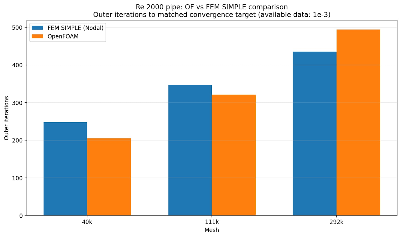
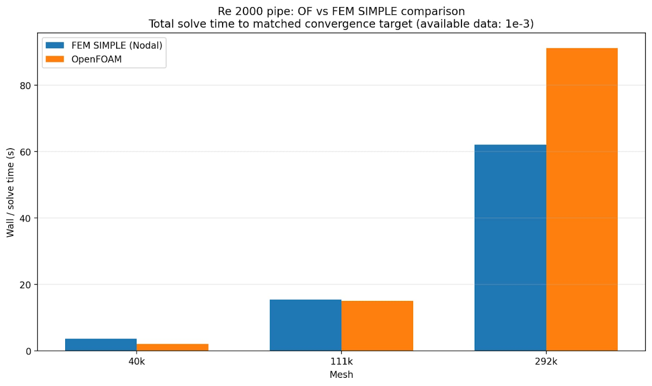
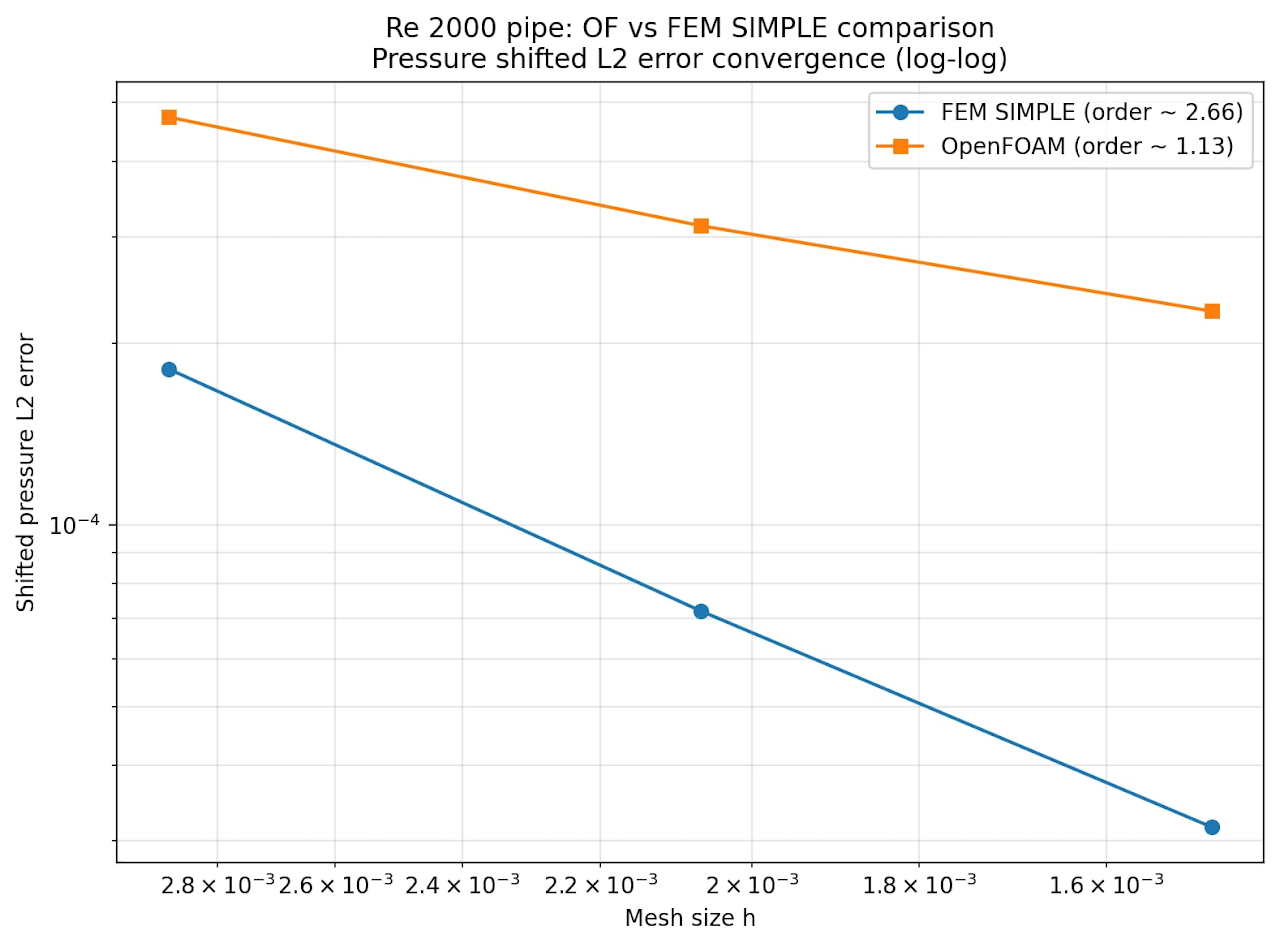
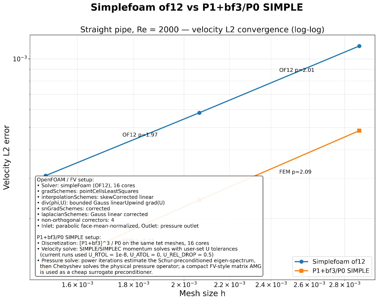
<p class="zfr3Q CDt4Ke " dir="ltr"><span class="C9DxTc ">Straight-pipe tests were encouraging. In laminar Hagen-Poiseuille flow, including cases around Reynolds numbers 20 and 2000, the solver produced the expected pressure-gradient and velocity-profile convergence and compared well with a finite-volume SIMPLE reference. Those tests were important because they separated the basic mixed discretization and SIMPLE coupling from turbulence-model complications.</span></p>
</div>
</div>
</div>
</div>
</div>
</div>
</div>
</div>
</div>
</section>
<section id="h.48b84d2315451c26_158" class="yaqOZd">
<div class="mYVXT">
<div class="LS81yb VICjCf j5pSsc db35Fc" tabindex="-1">
<div class="hJDwNd-AhqUyc-OiUrBf Ft7HRd-AhqUyc-OiUrBf purZT-AhqUyc-II5mzb ZcASvf-AhqUyc-II5mzb pSzOP-AhqUyc-qWD73c Ktthjf-AhqUyc-qWD73c JNdkSc SQVYQc yYI8W HQwdzb">
<div class="JNdkSc-SmKAyb LkDMRd">
<div class="">
<div class="oKdM2c ZZyype Kzv0Me">
<div id="h.48b84d2315451c26_155" class="hJDwNd-AhqUyc-OiUrBf Ft7HRd-AhqUyc-OiUrBf jXK9ad D2fZ2 zu5uec OjCsFc dmUFtb">
<div class="jXK9ad-SmKAyb">
<div class="tyJCtd baZpAe">
<div class="t3iYD">
<figure class="CENy8b post__image"><img loading="lazy" role="img" src="https://jade-speculoos-11a861.netlify.app/media/posts/6/9.png" alt="Figure 3: NodalS: Outer iterations for convergence vs OpenFOAM" width="1280" height="758" sizes="(max-width: 1920px) 100vw, 1920px" srcset="https://jade-speculoos-11a861.netlify.app/media/posts/6/responsive/9-xs.png 640w ,https://jade-speculoos-11a861.netlify.app/media/posts/6/responsive/9-sm.png 768w ,https://jade-speculoos-11a861.netlify.app/media/posts/6/responsive/9-md.png 1024w ,https://jade-speculoos-11a861.netlify.app/media/posts/6/responsive/9-lg.png 1366w ,https://jade-speculoos-11a861.netlify.app/media/posts/6/responsive/9-xl.png 1600w ,https://jade-speculoos-11a861.netlify.app/media/posts/6/responsive/9-2xl.png 1920w">
<figcaption><span class="C9DxTc ">Figure 3: NodalS: Outer iterations for convergence vs OpenFOAM</span></figcaption>
</figure>
</div>
</div>
</div>
</div>
</div>
<div class="oKdM2c ZZyype">
<div id="h.48b84d2315451c26_159" class="hJDwNd-AhqUyc-OiUrBf Ft7HRd-AhqUyc-OiUrBf jXK9ad D2fZ2 zu5uec wHaque g5GTcb">
<figure class="CENy8b post__image"><img loading="lazy" style="font-size: inherit;" role="img" src="https://jade-speculoos-11a861.netlify.app/media/posts/6/10.png" alt="Figure 4: NodalS wall time for convergence vs OpenFOAM" width="1280" height="758" sizes="(max-width: 1920px) 100vw, 1920px" srcset="https://jade-speculoos-11a861.netlify.app/media/posts/6/responsive/10-xs.png 640w ,https://jade-speculoos-11a861.netlify.app/media/posts/6/responsive/10-sm.png 768w ,https://jade-speculoos-11a861.netlify.app/media/posts/6/responsive/10-md.png 1024w ,https://jade-speculoos-11a861.netlify.app/media/posts/6/responsive/10-lg.png 1366w ,https://jade-speculoos-11a861.netlify.app/media/posts/6/responsive/10-xl.png 1600w ,https://jade-speculoos-11a861.netlify.app/media/posts/6/responsive/10-2xl.png 1920w">
<figcaption><span class="C9DxTc ">Figure 4: NodalS wall time for convergence vs OpenFOAM</span></figcaption>
</figure>
</div>
</div>
</div>
</div>
</div>
</div>
</div>
</section>
<section id="h.48b84d2315451c26_164" class="yaqOZd">
<div class="mYVXT">
<div class="LS81yb VICjCf j5pSsc db35Fc" tabindex="-1">
<div class="hJDwNd-AhqUyc-OiUrBf Ft7HRd-AhqUyc-OiUrBf purZT-AhqUyc-II5mzb ZcASvf-AhqUyc-II5mzb pSzOP-AhqUyc-qWD73c Ktthjf-AhqUyc-qWD73c JNdkSc SQVYQc yYI8W HQwdzb">
<div class="JNdkSc-SmKAyb LkDMRd">
<div class="">
<div class="oKdM2c ZZyype">
<div id="h.48b84d2315451c26_165" class="hJDwNd-AhqUyc-OiUrBf Ft7HRd-AhqUyc-OiUrBf jXK9ad D2fZ2 zu5uec wHaque g5GTcb">
<div class="jXK9ad-SmKAyb">
<div class="tyJCtd mGzaTb Depvyb baZpAe">
<figure class="post__image"><img loading="lazy" style="font-size: inherit;" role="img" src="https://jade-speculoos-11a861.netlify.app/media/posts/6/11.png" alt="Figure 5: Pressure error comparison vs OpenFOAM" width="1280" height="947" sizes="(max-width: 1920px) 100vw, 1920px" srcset="https://jade-speculoos-11a861.netlify.app/media/posts/6/responsive/11-xs.png 640w ,https://jade-speculoos-11a861.netlify.app/media/posts/6/responsive/11-sm.png 768w ,https://jade-speculoos-11a861.netlify.app/media/posts/6/responsive/11-md.png 1024w ,https://jade-speculoos-11a861.netlify.app/media/posts/6/responsive/11-lg.png 1366w ,https://jade-speculoos-11a861.netlify.app/media/posts/6/responsive/11-xl.png 1600w ,https://jade-speculoos-11a861.netlify.app/media/posts/6/responsive/11-2xl.png 1920w">
<figcaption><span class="C9DxTc ">Figure 5: Pressure error comparison vs OpenFOAM</span></figcaption>
</figure>
</div>
</div>
</div>
</div>
</div>
</div>
</div>
</div>
</div>
</section>
<section id="h.48b84d2315451c26_170" class="yaqOZd">
<div class="mYVXT">
<div class="LS81yb VICjCf j5pSsc db35Fc" tabindex="-1">
<div class="hJDwNd-AhqUyc-OiUrBf Ft7HRd-AhqUyc-OiUrBf purZT-AhqUyc-II5mzb ZcASvf-AhqUyc-II5mzb pSzOP-AhqUyc-qWD73c Ktthjf-AhqUyc-qWD73c JNdkSc SQVYQc yYI8W HQwdzb">
<div class="JNdkSc-SmKAyb LkDMRd">
<div class="">
<div class="oKdM2c ZZyype">
<div id="h.48b84d2315451c26_171" class="hJDwNd-AhqUyc-OiUrBf Ft7HRd-AhqUyc-OiUrBf jXK9ad D2fZ2 zu5uec wHaque g5GTcb">
<div class="jXK9ad-SmKAyb">
<div class="tyJCtd mGzaTb Depvyb baZpAe">
<figure class="CENy8b post__image"><img loading="lazy" style="font-size: inherit;" role="img" src="https://jade-speculoos-11a861.netlify.app/media/posts/6/12.png" alt="Figure 6: Velocity error vs OpenFOAM (alongwith scheme descriptions)" width="1280" height="1019" sizes="(max-width: 1920px) 100vw, 1920px" srcset="https://jade-speculoos-11a861.netlify.app/media/posts/6/responsive/12-xs.png 640w ,https://jade-speculoos-11a861.netlify.app/media/posts/6/responsive/12-sm.png 768w ,https://jade-speculoos-11a861.netlify.app/media/posts/6/responsive/12-md.png 1024w ,https://jade-speculoos-11a861.netlify.app/media/posts/6/responsive/12-lg.png 1366w ,https://jade-speculoos-11a861.netlify.app/media/posts/6/responsive/12-xl.png 1600w ,https://jade-speculoos-11a861.netlify.app/media/posts/6/responsive/12-2xl.png 1920w">
<figcaption><span class="C9DxTc ">Figure 6: Velocity error vs OpenFOAM (alongwith scheme descriptions)</span></figcaption>
</figure>
</div>
</div>
</div>
</div>
</div>
</div>
</div>
</div>
</div>
</section>
<section id="h.48b84d2315451c26_176" class="yaqOZd">
<div class="mYVXT">
<div class="LS81yb VICjCf j5pSsc db35Fc" tabindex="-1">
<div class="hJDwNd-AhqUyc-OiUrBf Ft7HRd-AhqUyc-OiUrBf purZT-AhqUyc-II5mzb ZcASvf-AhqUyc-II5mzb pSzOP-AhqUyc-qWD73c Ktthjf-AhqUyc-qWD73c JNdkSc SQVYQc yYI8W HQwdzb">
<div class="JNdkSc-SmKAyb LkDMRd">
<div class="">
<div class="oKdM2c ZZyype">
<div id="h.48b84d2315451c26_177" class="hJDwNd-AhqUyc-OiUrBf Ft7HRd-AhqUyc-OiUrBf jXK9ad D2fZ2 zu5uec wHaque g5GTcb">
<div class="jXK9ad-SmKAyb">
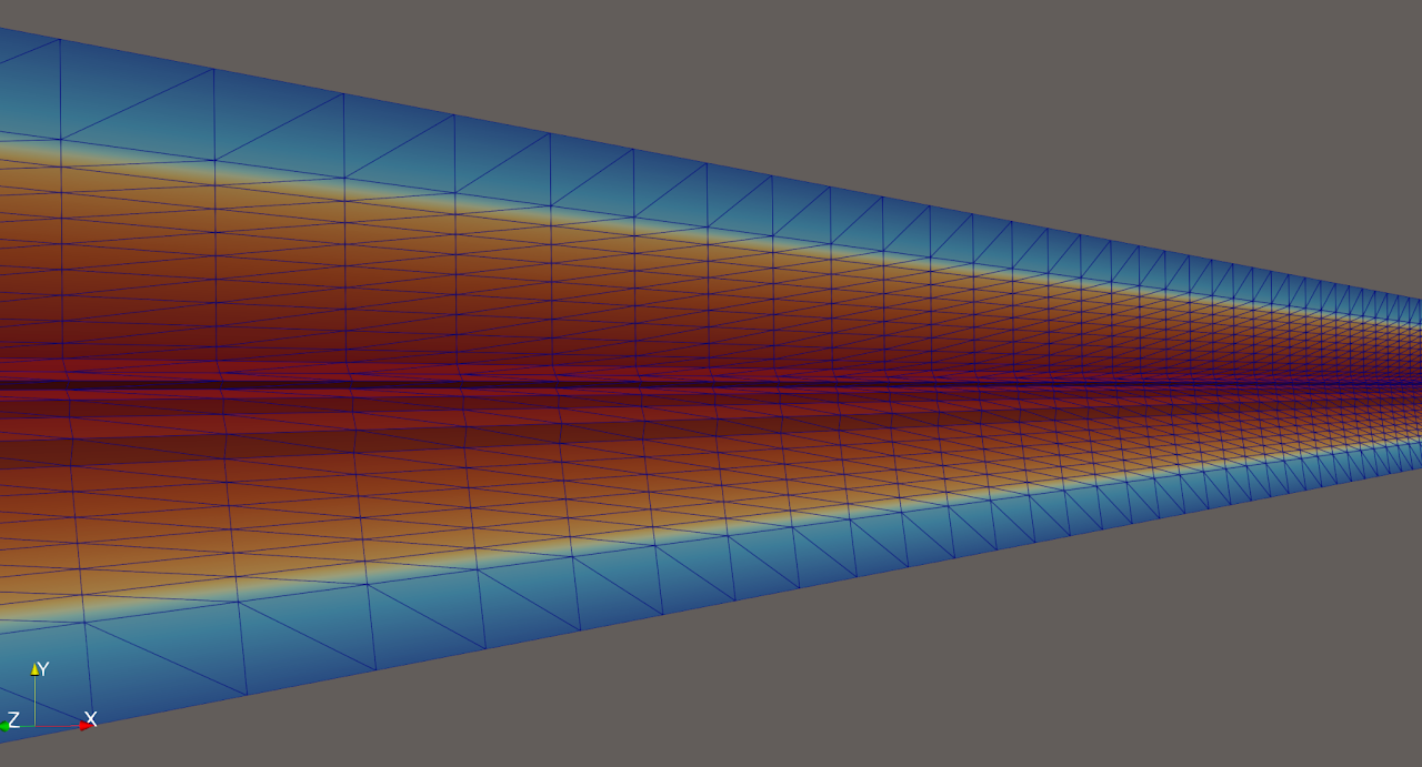
<div class="tyJCtd mGzaTb Depvyb baZpAe"><span style="font-size: inherit;">For the next step towards turbulent flow we aimed to produce our values for the VMFL003 Ansys benchmark. This benchmark uses a pipe that 500 diameters long and it exposed a geometric weakness rather than a fundamental algebraic one. Trying to represent its wall layer with tetrahedra while keeping the overall cell count manageable required strongly stretched elements. In that mesh family the tetrahedral formulation developed sliver-like cells and the turbulent pressure-drop error rose to roughly nine percent.</span></div>
</div>
</div>
</div>
</div>
</div>
</div>
</div>
</div>
</section>
<section id="h.48b84d2315451c26_186" class="yaqOZd">
<div class="mYVXT">
<div class="LS81yb VICjCf j5pSsc db35Fc" tabindex="-1">
<div class="hJDwNd-AhqUyc-OiUrBf Ft7HRd-AhqUyc-OiUrBf purZT-AhqUyc-II5mzb ZcASvf-AhqUyc-II5mzb pSzOP-AhqUyc-qWD73c Ktthjf-AhqUyc-qWD73c JNdkSc SQVYQc yYI8W HQwdzb">
<div class="JNdkSc-SmKAyb LkDMRd">
<div class="">
<div class="oKdM2c ZZyype Kzv0Me">
<div id="h.48b84d2315451c26_183" class="hJDwNd-AhqUyc-OiUrBf Ft7HRd-AhqUyc-OiUrBf jXK9ad D2fZ2 zu5uec OjCsFc dmUFtb">
<div class="jXK9ad-SmKAyb">
<div class="tyJCtd baZpAe">
<div class="t3iYD">
<figure class="CENy8b post__image"><img loading="lazy" role="img" src="https://jade-speculoos-11a861.netlify.app/media/posts/6/13.png" alt="Figure 7: The tet mesh used for turbulent flow computations (mid plane cross section of the pipe geometry)" width="1280" height="691" sizes="(max-width: 1920px) 100vw, 1920px" srcset="https://jade-speculoos-11a861.netlify.app/media/posts/6/responsive/13-xs.png 640w ,https://jade-speculoos-11a861.netlify.app/media/posts/6/responsive/13-sm.png 768w ,https://jade-speculoos-11a861.netlify.app/media/posts/6/responsive/13-md.png 1024w ,https://jade-speculoos-11a861.netlify.app/media/posts/6/responsive/13-lg.png 1366w ,https://jade-speculoos-11a861.netlify.app/media/posts/6/responsive/13-xl.png 1600w ,https://jade-speculoos-11a861.netlify.app/media/posts/6/responsive/13-2xl.png 1920w">
<figcaption><span class="C9DxTc ">Figure 7: The tet mesh used for turbulent flow computations (mid plane cross section of the pipe geometry)</span></figcaption>
</figure>
</div>
</div>
</div>
</div>
</div>
<div class="oKdM2c ZZyype">
<div id="h.48b84d2315451c26_187" class="hJDwNd-AhqUyc-OiUrBf Ft7HRd-AhqUyc-OiUrBf jXK9ad D2fZ2 zu5uec wHaque g5GTcb">
<div class="jXK9ad-SmKAyb">
<div class="tyJCtd mGzaTb Depvyb baZpAe"><span style="font-size: inherit;">That result motivated a change of element shape rather than a change of the basic solver idea: preserve cellwise discontinuous pressure and shared face velocity enrichment, but move to hexahedra whose long axial aspect ratios remain much better conditioned.</span></div>
</div>
</div>
</div>
</div>
</div>
</div>
</div>
</div>
</section>
<section id="h.48b84d2315451c26_196" class="yaqOZd">
<div class="mYVXT">
<div class="LS81yb VICjCf j5pSsc db35Fc" tabindex="-1">
<div class="hJDwNd-AhqUyc-uQSCkd Ft7HRd-AhqUyc-uQSCkd purZT-AhqUyc-II5mzb ZcASvf-AhqUyc-II5mzb pSzOP-AhqUyc-qWD73c Ktthjf-AhqUyc-qWD73c JNdkSc SQVYQc">
<div class="JNdkSc-SmKAyb LkDMRd">
<div class="">
<div class="oKdM2c ZZyype Kzv0Me">
<div id="h.48b84d2315451c26_193" class="hJDwNd-AhqUyc-uQSCkd Ft7HRd-AhqUyc-uQSCkd jXK9ad D2fZ2 zu5uec OjCsFc dmUFtb wHaque g5GTcb">
<div class="jXK9ad-SmKAyb">
<div class="tyJCtd mGzaTb Depvyb baZpAe">
<h2 class="CjVfdc"><span class="C9DxTc ">5. Hex analogue: Q1+BF2/Q0</span></h2>
<h3 id="h.5u9kwege7t83_l" class="zfr3Q OmQG5e CDt4Ke " dir="ltr"></h3>
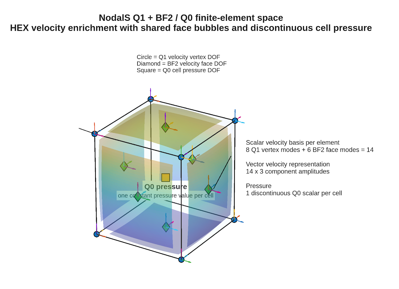
<p class="zfr3Q CDt4Ke " dir="ltr"><span class="C9DxTc ">The strict-hex version of NodalS uses eight standard trilinear Q1 vertex modes plus six shared quadrilateral-face bubble modes per element. Each scalar velocity component therefore has 14 local modes, while pressure remains one discontinuous Q0 value per hex cell. (see figure 3)</span></p>
</div>
</div>
</div>
</div>
</div>
</div>
</div>
</div>
</div>
</section>
<section id="h.48b84d2315451c26_200" class="yaqOZd">
<div class="mYVXT">
<div class="LS81yb VICjCf j5pSsc db35Fc" tabindex="-1">
<div class="hJDwNd-AhqUyc-OiUrBf Ft7HRd-AhqUyc-OiUrBf purZT-AhqUyc-II5mzb ZcASvf-AhqUyc-II5mzb pSzOP-AhqUyc-qWD73c Ktthjf-AhqUyc-qWD73c JNdkSc SQVYQc yYI8W HQwdzb">
<div class="JNdkSc-SmKAyb LkDMRd">
<div class="">
<div class="oKdM2c ZZyype Kzv0Me">
<div id="h.48b84d2315451c26_197" class="hJDwNd-AhqUyc-OiUrBf Ft7HRd-AhqUyc-OiUrBf jXK9ad D2fZ2 zu5uec OjCsFc dmUFtb">
<div class="jXK9ad-SmKAyb">
<div class="tyJCtd baZpAe">
<div class="t3iYD">
<figure class="CENy8b post__image"><img loading="lazy" role="img" src="https://jade-speculoos-11a861.netlify.app/media/posts/6/14.png" alt="Strict-hex mixed element used for the turbulent-pipe work" width="1280" height="161" sizes="(max-width: 1920px) 100vw, 1920px" srcset="https://jade-speculoos-11a861.netlify.app/media/posts/6/responsive/14-xs.png 640w ,https://jade-speculoos-11a861.netlify.app/media/posts/6/responsive/14-sm.png 768w ,https://jade-speculoos-11a861.netlify.app/media/posts/6/responsive/14-md.png 1024w ,https://jade-speculoos-11a861.netlify.app/media/posts/6/responsive/14-lg.png 1366w ,https://jade-speculoos-11a861.netlify.app/media/posts/6/responsive/14-xl.png 1600w ,https://jade-speculoos-11a861.netlify.app/media/posts/6/responsive/14-2xl.png 1920w">
<figcaption><span class="C9DxTc ">Strict-hex mixed element used for the turbulent-pipe work</span></figcaption>
</figure>
</div>
</div>
</div>
</div>
</div>
</div>
</div>
</div>
</div>
</div>
</section>
<section id="h.48b84d2315451c26_206" class="yaqOZd">
<div class="mYVXT">
<div class="LS81yb VICjCf j5pSsc db35Fc" tabindex="-1">
<div class="hJDwNd-AhqUyc-uQSCkd Ft7HRd-AhqUyc-uQSCkd purZT-AhqUyc-II5mzb ZcASvf-AhqUyc-II5mzb pSzOP-AhqUyc-qWD73c Ktthjf-AhqUyc-qWD73c JNdkSc SQVYQc">
<div class="JNdkSc-SmKAyb LkDMRd">
<div class="">
<div class="oKdM2c ZZyype Kzv0Me">
<div id="h.48b84d2315451c26_203" class="hJDwNd-AhqUyc-uQSCkd Ft7HRd-AhqUyc-uQSCkd jXK9ad D2fZ2 zu5uec OjCsFc dmUFtb wHaque g5GTcb">
<div class="jXK9ad-SmKAyb">
<div class="tyJCtd mGzaTb Depvyb baZpAe">
<p class="zfr3Q CDt4Ke " dir="ltr"><span class="C9DxTc ">The intent is directly analogous to the tetrahedral element: the Q1 part provides the continuous low-order velocity field and the six face modes supply the additional flux-carrying directions needed by the mixed pressure coupling. The bubbles are shared face entities, not independent interior bubbles duplicated by each neighbouring cell.</span></p>
</div>
</div>
</div>
</div>
</div>
</div>
</div>
</div>
</div>
</section>
<section id="h.48b84d2315451c26_210" class="yaqOZd">
<div class="mYVXT">
<div class="LS81yb VICjCf j5pSsc db35Fc" tabindex="-1">
<div class="hJDwNd-AhqUyc-OiUrBf Ft7HRd-AhqUyc-OiUrBf purZT-AhqUyc-II5mzb ZcASvf-AhqUyc-II5mzb pSzOP-AhqUyc-qWD73c Ktthjf-AhqUyc-qWD73c JNdkSc SQVYQc yYI8W HQwdzb">
<div class="JNdkSc-SmKAyb LkDMRd">
<div class="">
<div class="oKdM2c ZZyype Kzv0Me">
<div id="h.48b84d2315451c26_207" class="hJDwNd-AhqUyc-OiUrBf Ft7HRd-AhqUyc-OiUrBf jXK9ad D2fZ2 zu5uec OjCsFc dmUFtb">
<div class="jXK9ad-SmKAyb">
<div class="tyJCtd baZpAe">
<div class="t3iYD">
<figure class="CENy8b post__image"><img loading="lazy" role="img" src="https://jade-speculoos-11a861.netlify.app/media/posts/6/15.png" alt="Figure 8: The hex mesh used for turbulent flow computations (mid plane cut section)" width="1280" height="691" sizes="(max-width: 1920px) 100vw, 1920px" srcset="https://jade-speculoos-11a861.netlify.app/media/posts/6/responsive/15-xs.png 640w ,https://jade-speculoos-11a861.netlify.app/media/posts/6/responsive/15-sm.png 768w ,https://jade-speculoos-11a861.netlify.app/media/posts/6/responsive/15-md.png 1024w ,https://jade-speculoos-11a861.netlify.app/media/posts/6/responsive/15-lg.png 1366w ,https://jade-speculoos-11a861.netlify.app/media/posts/6/responsive/15-xl.png 1600w ,https://jade-speculoos-11a861.netlify.app/media/posts/6/responsive/15-2xl.png 1920w">
<figcaption><span class="C9DxTc ">Figure 8: The hex mesh used for turbulent flow computations (mid plane cut section)</span></figcaption>
</figure>
</div>
</div>
</div>
</div>
</div>
</div>
</div>
</div>
<div class="hJDwNd-AhqUyc-ibL1re Ft7HRd-AhqUyc-ibL1re JNdkSc SQVYQc L6cTce-purZT L6cTce-pSzOP">
<div class="JNdkSc-SmKAyb LkDMRd">
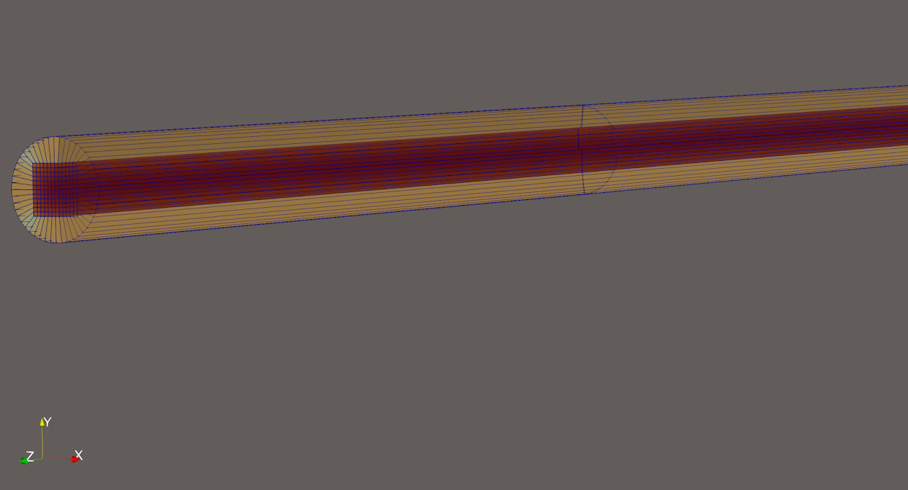
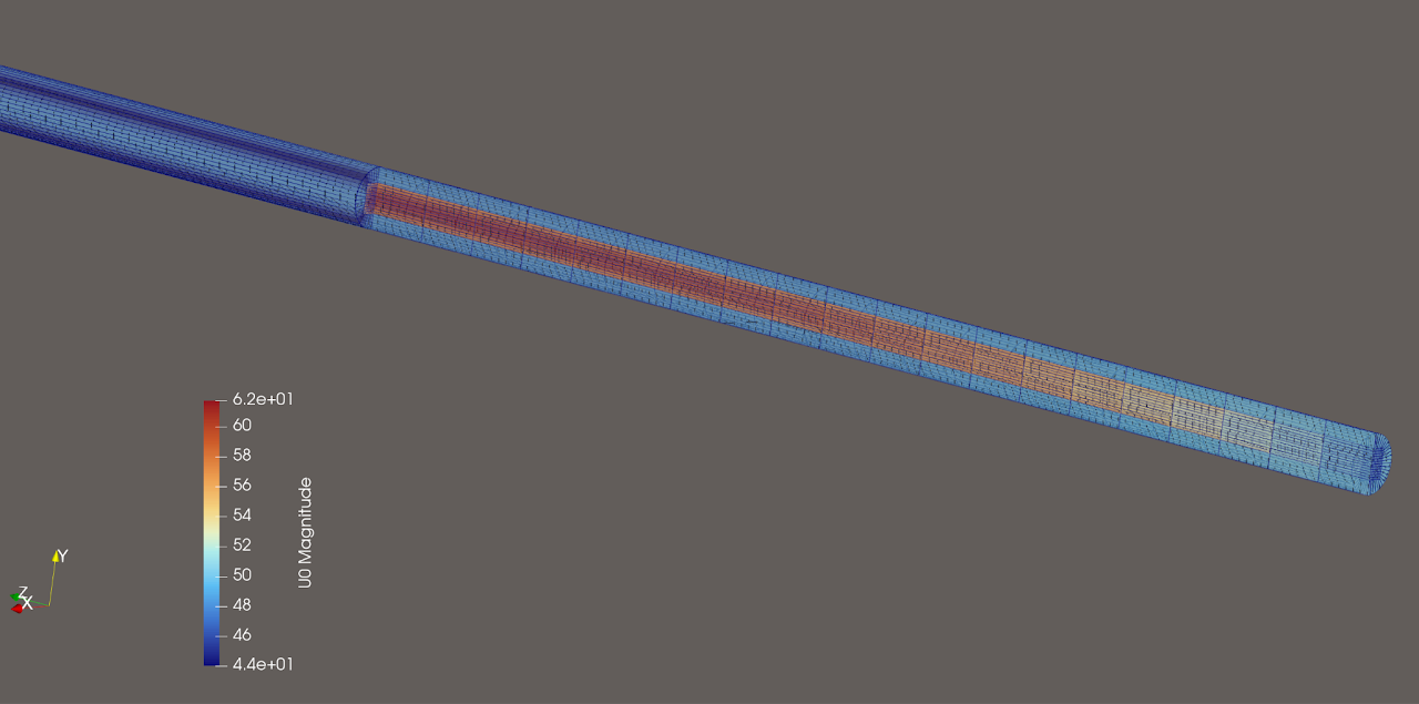
<div class=""><span style="font-size: inherit;">The VMFL003 article mesh is deliberately coarse: an O-grid with 192 hexahedra in each cross-section and only 68 axial layers, for 13,056 cells in a 500D pipe. The first 20D uses 20 layers of length 1D, followed by 48 long layers of 10D. This is exactly the kind of geometry for which elongated, aligned hexes are appealing.</span></div>
</div>
</div>
</div>
</div>
</section>
<section id="h.48b84d2315451c26_220" class="yaqOZd">
<div class="mYVXT">
<div class="LS81yb VICjCf j5pSsc db35Fc" tabindex="-1">
<div class="hJDwNd-AhqUyc-uQSCkd Ft7HRd-AhqUyc-uQSCkd purZT-AhqUyc-II5mzb ZcASvf-AhqUyc-II5mzb pSzOP-AhqUyc-qWD73c Ktthjf-AhqUyc-qWD73c JNdkSc SQVYQc">
<div class="JNdkSc-SmKAyb LkDMRd">
<div class="">
<div class="oKdM2c ZZyype Kzv0Me">
<div id="h.48b84d2315451c26_217" class="hJDwNd-AhqUyc-uQSCkd Ft7HRd-AhqUyc-uQSCkd jXK9ad D2fZ2 zu5uec OjCsFc dmUFtb wHaque g5GTcb">
<div class="jXK9ad-SmKAyb">
<div class="tyJCtd mGzaTb Depvyb baZpAe">
<h2 class="CjVfdc"><span class="C9DxTc ">6. Cheap momentum smoothing with Chebyshev-Jacobi</span></h2>
<h3 id="h.7q743ep03q3x_l" class="zfr3Q OmQG5e CDt4Ke " dir="ltr"></h3>
<p class="zfr3Q CDt4Ke " dir="ltr"><span class="C9DxTc ">A diagonal preconditioner is attractive for memory and parallelism, but plain Jacobi can be a poor smoother when the momentum operator becomes strongly anisotropic or badly scaled. The NodalS hex branch therefore uses higher-degree Chebyshev smoothing on top of Jacobi in PETSc's multigrid hierarchy.</span></p>
</div>
</div>
</div>
</div>
</div>
</div>
</div>
</div>
</div>
</section>
<section id="h.48b84d2315451c26_224" class="yaqOZd">
<div class="mYVXT">
<div class="LS81yb VICjCf j5pSsc db35Fc" tabindex="-1">
<div class="hJDwNd-AhqUyc-OiUrBf Ft7HRd-AhqUyc-OiUrBf purZT-AhqUyc-II5mzb ZcASvf-AhqUyc-II5mzb pSzOP-AhqUyc-qWD73c Ktthjf-AhqUyc-qWD73c JNdkSc SQVYQc yYI8W HQwdzb">
<div class="JNdkSc-SmKAyb LkDMRd">
<div class="">
<div class="oKdM2c ZZyype Kzv0Me">
<div id="h.48b84d2315451c26_221" class="hJDwNd-AhqUyc-OiUrBf Ft7HRd-AhqUyc-OiUrBf jXK9ad D2fZ2 zu5uec OjCsFc dmUFtb">
<div class="jXK9ad-SmKAyb">
<div class="tyJCtd baZpAe">
<div class="t3iYD">
<figure class="post__image"><img loading="lazy" role="img" src="https://jade-speculoos-11a861.netlify.app/media/posts/6/16.png" alt="Conceptual Chebyshev-accelerated Jacobi iteration" width="1280" height="161" sizes="(max-width: 1920px) 100vw, 1920px" srcset="https://jade-speculoos-11a861.netlify.app/media/posts/6/responsive/16-xs.png 640w ,https://jade-speculoos-11a861.netlify.app/media/posts/6/responsive/16-sm.png 768w ,https://jade-speculoos-11a861.netlify.app/media/posts/6/responsive/16-md.png 1024w ,https://jade-speculoos-11a861.netlify.app/media/posts/6/responsive/16-lg.png 1366w ,https://jade-speculoos-11a861.netlify.app/media/posts/6/responsive/16-xl.png 1600w ,https://jade-speculoos-11a861.netlify.app/media/posts/6/responsive/16-2xl.png 1920w">
<figcaption><span class="C9DxTc ">Conceptual Chebyshev-accelerated Jacobi iteration</span></figcaption>
</figure>
</div>
</div>
</div>
</div>
</div>
</div>
</div>
</div>
<div class="hJDwNd-AhqUyc-ibL1re Ft7HRd-AhqUyc-ibL1re JNdkSc SQVYQc L6cTce-purZT L6cTce-pSzOP">
<div class="JNdkSc-SmKAyb LkDMRd">
<div class=""><span style="font-size: inherit;">The practical advantage is that Chebyshev iteration needs only repeated sparse operator applications and diagonal scaling once useful spectral bounds are available. PETSc can estimate the relevant eigenvalue range and then apply a polynomial that damps the unwanted part of the spectrum more effectively than one Jacobi step.</span></div>
</div>
</div>
</div>
</div>
</section>
<section id="h.48b84d2315451c26_230" class="yaqOZd">
<div class="mYVXT">
<div class="LS81yb VICjCf j5pSsc db35Fc" tabindex="-1">
<div class="hJDwNd-AhqUyc-uQSCkd Ft7HRd-AhqUyc-uQSCkd purZT-AhqUyc-II5mzb ZcASvf-AhqUyc-II5mzb pSzOP-AhqUyc-qWD73c Ktthjf-AhqUyc-qWD73c JNdkSc SQVYQc">
<div class="JNdkSc-SmKAyb LkDMRd">
<div class="">
<div class="oKdM2c ZZyype Kzv0Me">
<div id="h.48b84d2315451c26_227" class="hJDwNd-AhqUyc-uQSCkd Ft7HRd-AhqUyc-uQSCkd jXK9ad D2fZ2 zu5uec OjCsFc dmUFtb wHaque g5GTcb">
<div class="jXK9ad-SmKAyb">
<div class="tyJCtd mGzaTb Depvyb baZpAe">
<p class="zfr3Q CDt4Ke " dir="ltr"><span class="C9DxTc ">This became especially interesting in the turbulent runs. Plug, parabolic, and one-seventh-power-law inlet profiles could initially produce a difficult pressure/momentum transient with high Krylov iteration counts. Once the nonlinear state passed the steep entrance/start-up phase, the linear solves became much easier and the overall SIMPLE iteration converged. Interestingly for some cases this multigrid configuration led to much less iteration of the outer conjugate gradient than the conjugate gradient in OpenFOAM which was preconditioned with a gauss siedel based OpenFOAM GAMG.</span></p>
<p class="zfr3Q CDt4Ke " dir="ltr"><span class="C9DxTc ">However, this is a problem-specific observation, not a general robustness claim. The VMFL003 geometry is strongly aligned and the present wall model is specialized to a straight circular pipe. Still, the experiment is a positive sign for low-memory FE pressure-correction solvers built around sparse operator applications on a GPU.</span></p>
</div>
</div>
</div>
</div>
</div>
</div>
</div>
</div>
</div>
</section>
<section id="h.48b84d2315451c26_234" class="yaqOZd">
<div class="mYVXT">
<div class="LS81yb VICjCf j5pSsc db35Fc" tabindex="-1">
<div class="hJDwNd-AhqUyc-uQSCkd Ft7HRd-AhqUyc-uQSCkd purZT-AhqUyc-II5mzb ZcASvf-AhqUyc-II5mzb pSzOP-AhqUyc-qWD73c Ktthjf-AhqUyc-qWD73c JNdkSc SQVYQc">
<div class="JNdkSc-SmKAyb LkDMRd">
<div class="">
<div class="oKdM2c ZZyype Kzv0Me">
<div id="h.48b84d2315451c26_231" class="hJDwNd-AhqUyc-uQSCkd Ft7HRd-AhqUyc-uQSCkd jXK9ad D2fZ2 zu5uec OjCsFc dmUFtb wHaque g5GTcb">
<div class="jXK9ad-SmKAyb">
<div class="tyJCtd mGzaTb Depvyb baZpAe">
<h2 class="CjVfdc"><span class="C9DxTc ">7. Mixing length model</span></h2>
<h3 id="h.hzn3ntcour7m_l" class="zfr3Q OmQG5e CDt4Ke " dir="ltr"></h3>
<p class="zfr3Q CDt4Ke " dir="ltr"><span class="C9DxTc ">The turbulent-pipe solver was kept deliberately straightforward and simple for this elementary turbulence verification. This branch does not solve k, epsilon, omega, or any other transported turbulence variable. It uses a Nikuradse mixing-length closure evaluated at the volume quadrature points from the current velocity field.</span></p>
</div>
</div>
</div>
</div>
</div>
</div>
</div>
</div>
</div>
</section>
<section id="h.48b84d2315451c26_238" class="yaqOZd">
<div class="mYVXT">
<div class="LS81yb VICjCf j5pSsc db35Fc" tabindex="-1">
<div class="hJDwNd-AhqUyc-OiUrBf Ft7HRd-AhqUyc-OiUrBf purZT-AhqUyc-II5mzb ZcASvf-AhqUyc-II5mzb pSzOP-AhqUyc-qWD73c Ktthjf-AhqUyc-qWD73c JNdkSc SQVYQc yYI8W HQwdzb">
<div class="JNdkSc-SmKAyb LkDMRd">
<div class="">
<div class="oKdM2c ZZyype Kzv0Me">
<div id="h.48b84d2315451c26_235" class="hJDwNd-AhqUyc-OiUrBf Ft7HRd-AhqUyc-OiUrBf jXK9ad D2fZ2 zu5uec OjCsFc dmUFtb">
<div class="jXK9ad-SmKAyb">
<div class="tyJCtd baZpAe">
<div class="t3iYD">
<figure class="CENy8b post__image"><img loading="lazy" role="img" src="https://jade-speculoos-11a861.netlify.app/media/posts/6/17.png" alt="Nikuradse pipe mixing length and algebraic eddy viscosity" width="1280" height="218" sizes="(max-width: 1920px) 100vw, 1920px" srcset="https://jade-speculoos-11a861.netlify.app/media/posts/6/responsive/17-xs.png 640w ,https://jade-speculoos-11a861.netlify.app/media/posts/6/responsive/17-sm.png 768w ,https://jade-speculoos-11a861.netlify.app/media/posts/6/responsive/17-md.png 1024w ,https://jade-speculoos-11a861.netlify.app/media/posts/6/responsive/17-lg.png 1366w ,https://jade-speculoos-11a861.netlify.app/media/posts/6/responsive/17-xl.png 1600w ,https://jade-speculoos-11a861.netlify.app/media/posts/6/responsive/17-2xl.png 1920w">
<figcaption><span class="C9DxTc ">Nikuradse pipe mixing length and algebraic eddy viscosity</span></figcaption>
</figure>
</div>
</div>
</div>
</div>
</div>
</div>
</div>
</div>
</div>
</div>
</section>
<section id="h.48b84d2315451c26_244" class="yaqOZd">
<div class="mYVXT">
<div class="LS81yb VICjCf j5pSsc db35Fc" tabindex="-1">
<div class="hJDwNd-AhqUyc-uQSCkd Ft7HRd-AhqUyc-uQSCkd purZT-AhqUyc-II5mzb ZcASvf-AhqUyc-II5mzb pSzOP-AhqUyc-qWD73c Ktthjf-AhqUyc-qWD73c JNdkSc SQVYQc">
<div class="JNdkSc-SmKAyb LkDMRd">
<div class="">
<div class="oKdM2c ZZyype Kzv0Me">
<div id="h.48b84d2315451c26_241" class="hJDwNd-AhqUyc-uQSCkd Ft7HRd-AhqUyc-uQSCkd jXK9ad D2fZ2 zu5uec OjCsFc dmUFtb wHaque g5GTcb">
<div class="jXK9ad-SmKAyb">
<div class="tyJCtd mGzaTb Depvyb baZpAe">
<p class="zfr3Q CDt4Ke " dir="ltr"><span class="C9DxTc ">The turbulent viscosity is therefore an algebraic consequence of the lagged SIMPLE velocity gradient. The accepted implementation updates the turbulent diffusion incrementally from one SIMPLE state to the next rather than storing a second full momentum matrix or a persistent cell-by-quadrature turbulent-viscosity field.</span></p>
<p class="zfr3Q CDt4Ke " dir="ltr"><span class="C9DxTc ">The calculation is initialized from a plug velocity. Because an exact plug has almost no interior strain, the initial volume eddy viscosity is nearly zero. The wall treatment supplies shear first; the velocity profile then develops, nonzero strain appears, and the algebraic turbulent viscosity emerges naturally in subsequent SIMPLE iterations.</span></p>
</div>
</div>
</div>
</div>
</div>
</div>
</div>
</div>
</div>
</section>
<section id="h.48b84d2315451c26_248" class="yaqOZd">
<div class="mYVXT">
<div class="LS81yb VICjCf j5pSsc db35Fc" tabindex="-1">
<div class="hJDwNd-AhqUyc-uQSCkd Ft7HRd-AhqUyc-uQSCkd purZT-AhqUyc-II5mzb ZcASvf-AhqUyc-II5mzb pSzOP-AhqUyc-qWD73c Ktthjf-AhqUyc-qWD73c JNdkSc SQVYQc">
<div class="JNdkSc-SmKAyb LkDMRd">
<div class="">
<div class="oKdM2c ZZyype Kzv0Me">
<div id="h.48b84d2315451c26_245" class="hJDwNd-AhqUyc-uQSCkd Ft7HRd-AhqUyc-uQSCkd jXK9ad D2fZ2 zu5uec OjCsFc dmUFtb wHaque g5GTcb">
<div class="jXK9ad-SmKAyb">
<div class="tyJCtd mGzaTb Depvyb baZpAe">
<h2 class="CjVfdc"><span class="C9DxTc ">8. A weak Spalding wall treatment</span></h2>
<h3 id="h.ebwv10l5aehe_l" class="zfr3Q OmQG5e CDt4Ke " dir="ltr"></h3>
<p class="zfr3Q CDt4Ke " dir="ltr"><span class="C9DxTc ">The wall model was one of the most important parts of the development. </span></p>
<p class="zfr3Q CDt4Ke " dir="ltr"><span class="C9DxTc ">The accepted hex implementation evaluates the full Q1+BF2 velocity at a geometrically defined off-wall point. For each wall quadrature point it moves inward to the wall-adjacent element's reference midplane, maps both points to physical space, computes the true radial wall-normal distance, and inverts the Spalding relation for friction velocity.</span></p>
</div>
</div>
</div>
</div>
</div>
</div>
</div>
</div>
</div>
</section>
<section id="h.48b84d2315451c26_252" class="yaqOZd">
<div class="mYVXT">
<div class="LS81yb VICjCf j5pSsc db35Fc" tabindex="-1">
<div class="hJDwNd-AhqUyc-OiUrBf Ft7HRd-AhqUyc-OiUrBf purZT-AhqUyc-II5mzb ZcASvf-AhqUyc-II5mzb pSzOP-AhqUyc-qWD73c Ktthjf-AhqUyc-qWD73c JNdkSc SQVYQc yYI8W HQwdzb">
<div class="JNdkSc-SmKAyb LkDMRd">
<div class="">
<div class="oKdM2c ZZyype Kzv0Me">
<div id="h.48b84d2315451c26_249" class="hJDwNd-AhqUyc-OiUrBf Ft7HRd-AhqUyc-OiUrBf jXK9ad D2fZ2 zu5uec OjCsFc dmUFtb">
<div class="jXK9ad-SmKAyb">
<div class="tyJCtd baZpAe">
<div class="t3iYD">
<figure class="post__image"><img loading="lazy" src="https://jade-speculoos-11a861.netlify.app/media/posts/6/18.png" alt="Spalding relation used to obtain friction velocity and the weak wall coefficient" width="1280" height="218" sizes="(max-width: 1920px) 100vw, 1920px" srcset="https://jade-speculoos-11a861.netlify.app/media/posts/6/responsive/18-xs.png 640w ,https://jade-speculoos-11a861.netlify.app/media/posts/6/responsive/18-sm.png 768w ,https://jade-speculoos-11a861.netlify.app/media/posts/6/responsive/18-md.png 1024w ,https://jade-speculoos-11a861.netlify.app/media/posts/6/responsive/18-lg.png 1366w ,https://jade-speculoos-11a861.netlify.app/media/posts/6/responsive/18-xl.png 1600w ,https://jade-speculoos-11a861.netlify.app/media/posts/6/responsive/18-2xl.png 1920w">
<figcaption><span class="C9DxTc ">Spalding relation used to obtain friction velocity and the weak wall coefficient</span></figcaption>
</figure>
<span class="C9DxTc ">The resulting coefficient acts as a weak streamwise wall traction. For this straight z-aligned pipe, the two cross-stream velocity components are strongly clamped while the axial component is left free to respond to the wall model. This should therefore be described as a pipe-specific weak tangential wall treatment, not yet as a generic arbitrary-wall implementation.</span></div>
</div>
</div>
</div>
</div>
</div>
</div>
</div>
</div>
</div>
</section>
<section id="h.48b84d2315451c26_258" class="yaqOZd">
<div class="mYVXT">
<div class="LS81yb VICjCf j5pSsc db35Fc" tabindex="-1">
<div class="hJDwNd-AhqUyc-uQSCkd Ft7HRd-AhqUyc-uQSCkd purZT-AhqUyc-II5mzb ZcASvf-AhqUyc-II5mzb pSzOP-AhqUyc-qWD73c Ktthjf-AhqUyc-qWD73c JNdkSc SQVYQc">
<div class="JNdkSc-SmKAyb LkDMRd">
<div class="">
<div class="oKdM2c ZZyype Kzv0Me">
<div id="h.48b84d2315451c26_255" class="hJDwNd-AhqUyc-uQSCkd Ft7HRd-AhqUyc-uQSCkd jXK9ad D2fZ2 zu5uec OjCsFc dmUFtb wHaque g5GTcb">
<div class="jXK9ad-SmKAyb">
<div class="tyJCtd mGzaTb Depvyb baZpAe">
<p class="zfr3Q CDt4Ke " dir="ltr"><span class="C9DxTc ">An additional molecular Nitsche-consistency contribution was tested but eventually disabled in the accepted benchmark configuration because it duplicated part of the drag already represented by the Spalding traction. The final article case therefore uses the Spalding-derived wall traction without that extra molecular wall term.</span></p>
</div>
</div>
</div>
</div>
</div>
</div>
</div>
</div>
</div>
</section>
<section id="h.48b84d2315451c26_262" class="yaqOZd">
<div class="mYVXT">
<div class="LS81yb VICjCf j5pSsc db35Fc" tabindex="-1">
<div class="hJDwNd-AhqUyc-uQSCkd Ft7HRd-AhqUyc-uQSCkd purZT-AhqUyc-II5mzb ZcASvf-AhqUyc-II5mzb pSzOP-AhqUyc-qWD73c Ktthjf-AhqUyc-qWD73c JNdkSc SQVYQc">
<div class="JNdkSc-SmKAyb LkDMRd">
<div class="">
<div class="oKdM2c ZZyype Kzv0Me">
<div id="h.48b84d2315451c26_259" class="hJDwNd-AhqUyc-uQSCkd Ft7HRd-AhqUyc-uQSCkd jXK9ad D2fZ2 zu5uec OjCsFc dmUFtb wHaque g5GTcb">
<div class="jXK9ad-SmKAyb">
<div class="tyJCtd mGzaTb Depvyb baZpAe">
<h2 class="CjVfdc"><span class="C9DxTc ">9. The inlet-rim problem and the DG numerical trace</span></h2>
<h3 id="h.etsvyw9kd8jq_l" class="zfr3Q OmQG5e CDt4Ke " dir="ltr"></h3>
<p class="zfr3Q CDt4Ke " dir="ltr"><span class="C9DxTc ">A strong plug inlet creates a subtle incompatibility at the circular rim: the same globally continuous velocity entities are asked to satisfy both the inlet plug and the wall condition. The early strong-CG inlet could force the face modes to repair flux near the wall and produced a large artificial entrance pressure spike that did not disappear when the nonlinear tolerance was tightened.</span></p>
<p class="zfr3Q CDt4Ke " dir="ltr"><span class="C9DxTc ">The accepted solution was to keep the volume method continuous but impose the inlet as a DG-style numerical trace. The inlet Q1 and BF2 volume unknowns remain free; the prescribed external trace supplies the mass flux and the inflow state.</span></p>
</div>
</div>
</div>
</div>
</div>
</div>
</div>
</div>
</div>
</section>
<section id="h.48b84d2315451c26_266" class="yaqOZd">
<div class="mYVXT">
<div class="LS81yb VICjCf j5pSsc db35Fc" tabindex="-1">
<div class="hJDwNd-AhqUyc-OiUrBf Ft7HRd-AhqUyc-OiUrBf purZT-AhqUyc-II5mzb ZcASvf-AhqUyc-II5mzb pSzOP-AhqUyc-qWD73c Ktthjf-AhqUyc-qWD73c JNdkSc SQVYQc yYI8W HQwdzb">
<div class="JNdkSc-SmKAyb LkDMRd">
<div class="">
<div class="oKdM2c ZZyype Kzv0Me">
<div id="h.48b84d2315451c26_263" class="hJDwNd-AhqUyc-OiUrBf Ft7HRd-AhqUyc-OiUrBf jXK9ad D2fZ2 zu5uec OjCsFc dmUFtb">
<div class="jXK9ad-SmKAyb">
<div class="tyJCtd baZpAe">
<div class="t3iYD">
<figure class="CENy8b post__image"><img loading="lazy" role="img" src="https://jade-speculoos-11a861.netlify.app/media/posts/6/19.png" alt="Prescribed inlet trace used in the cellwise continuity operator" width="1280" height="161" sizes="(max-width: 1920px) 100vw, 1920px" srcset="https://jade-speculoos-11a861.netlify.app/media/posts/6/responsive/19-xs.png 640w ,https://jade-speculoos-11a861.netlify.app/media/posts/6/responsive/19-sm.png 768w ,https://jade-speculoos-11a861.netlify.app/media/posts/6/responsive/19-md.png 1024w ,https://jade-speculoos-11a861.netlify.app/media/posts/6/responsive/19-lg.png 1366w ,https://jade-speculoos-11a861.netlify.app/media/posts/6/responsive/19-xl.png 1600w ,https://jade-speculoos-11a861.netlify.app/media/posts/6/responsive/19-2xl.png 1920w">
<figcaption><span class="C9DxTc ">Prescribed inlet trace used in the cellwise continuity operator</span></figcaption>
</figure>
</div>
</div>
</div>
</div>
</div>
</div>
</div>
</div>
<div class="hJDwNd-AhqUyc-ibL1re Ft7HRd-AhqUyc-ibL1re JNdkSc SQVYQc L6cTce-purZT L6cTce-pSzOP">
<div class="JNdkSc-SmKAyb LkDMRd">
<div class=""><span style="font-size: inherit;">For first-layer cells, the Q0 continuity equation therefore uses the prescribed inlet flux rather than the finite-element volume trace. This fixes the total inlet mass flow exactly in the discrete continuity equation.</span></div>
</div>
</div>
</div>
</div>
</section>
<section id="h.48b84d2315451c26_272" class="yaqOZd">
<div class="mYVXT">
<div class="LS81yb VICjCf j5pSsc db35Fc" tabindex="-1">
<div class="hJDwNd-AhqUyc-uQSCkd Ft7HRd-AhqUyc-uQSCkd purZT-AhqUyc-II5mzb ZcASvf-AhqUyc-II5mzb pSzOP-AhqUyc-qWD73c Ktthjf-AhqUyc-qWD73c JNdkSc SQVYQc">
<div class="JNdkSc-SmKAyb LkDMRd">
<div class="">
<div class="oKdM2c ZZyype Kzv0Me">
<div id="h.48b84d2315451c26_269" class="hJDwNd-AhqUyc-uQSCkd Ft7HRd-AhqUyc-uQSCkd jXK9ad D2fZ2 zu5uec OjCsFc dmUFtb wHaque g5GTcb">
<div class="jXK9ad-SmKAyb">
<div class="tyJCtd mGzaTb Depvyb baZpAe">
<p class="zfr3Q CDt4Ke " dir="ltr"><span class="C9DxTc ">Convection receives a physical inflow/upwind correction using the prescribed trace, while viscous diffusion at the inlet is handled with a penalty-free nonsymmetric Nitsche term. This localized DG boundary idea removed most of the artificial entrance loss while leaving the rest of the velocity space continuous.</span></p>
</div>
</div>
</div>
</div>
</div>
</div>
</div>
</div>
</div>
</section>
<section id="h.48b84d2315451c26_276" class="yaqOZd">
<div class="mYVXT">
<div class="LS81yb VICjCf j5pSsc db35Fc" tabindex="-1">
<div class="hJDwNd-AhqUyc-OiUrBf Ft7HRd-AhqUyc-OiUrBf purZT-AhqUyc-II5mzb ZcASvf-AhqUyc-II5mzb pSzOP-AhqUyc-qWD73c Ktthjf-AhqUyc-qWD73c JNdkSc SQVYQc yYI8W HQwdzb">
<div class="JNdkSc-SmKAyb LkDMRd">
<div class="">
<div class="oKdM2c ZZyype Kzv0Me">
<div id="h.48b84d2315451c26_273" class="hJDwNd-AhqUyc-OiUrBf Ft7HRd-AhqUyc-OiUrBf jXK9ad D2fZ2 zu5uec OjCsFc dmUFtb">
<div class="jXK9ad-SmKAyb">
<div class="tyJCtd baZpAe">
<div class="t3iYD">
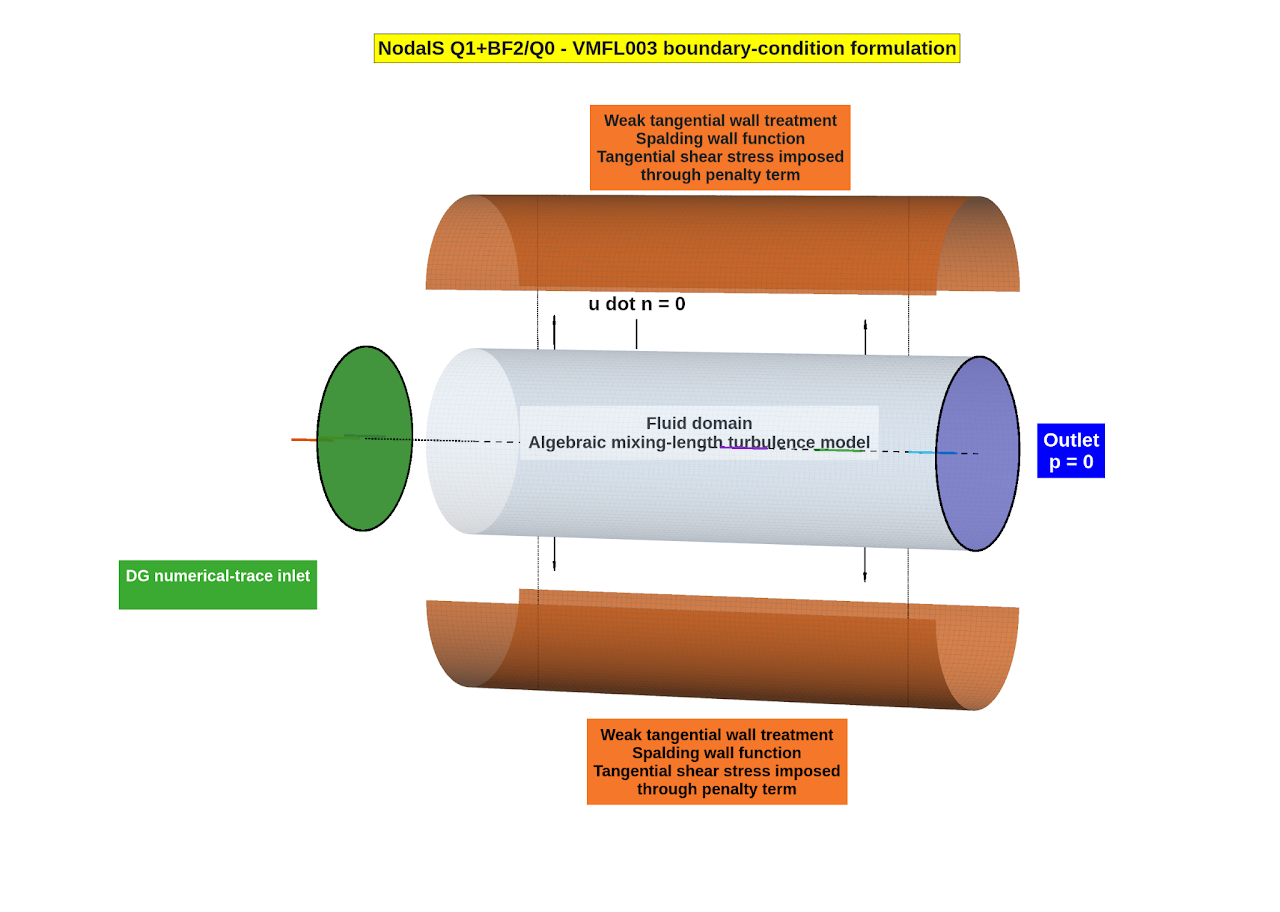
<figure class="CENy8b post__image"><img loading="lazy" role="img" src="https://jade-speculoos-11a861.netlify.app/media/posts/6/20.png" alt="Figure 9: Custom mixed finite-element SIMPLE solver - NodalS" width="1280" height="912" sizes="(max-width: 1920px) 100vw, 1920px" srcset="https://jade-speculoos-11a861.netlify.app/media/posts/6/responsive/20-xs.png 640w ,https://jade-speculoos-11a861.netlify.app/media/posts/6/responsive/20-sm.png 768w ,https://jade-speculoos-11a861.netlify.app/media/posts/6/responsive/20-md.png 1024w ,https://jade-speculoos-11a861.netlify.app/media/posts/6/responsive/20-lg.png 1366w ,https://jade-speculoos-11a861.netlify.app/media/posts/6/responsive/20-xl.png 1600w ,https://jade-speculoos-11a861.netlify.app/media/posts/6/responsive/20-2xl.png 1920w">
<figcaption><span class="C9DxTc ">Figure </span><span class="C9DxTc ">9</span><span class="C9DxTc ">: </span><span class="C9DxTc ">Custom mixed finite-element SIMPLE solver - NodalS</span></figcaption>
</figure>
</div>
</div>
</div>
</div>
</div>
</div>
</div>
</div>
</div>
</div>
</section>
<section id="h.48b84d2315451c26_282" class="yaqOZd">
<div class="mYVXT">
<div class="LS81yb VICjCf j5pSsc db35Fc" tabindex="-1">
<div class="hJDwNd-AhqUyc-OiUrBf Ft7HRd-AhqUyc-OiUrBf purZT-AhqUyc-II5mzb ZcASvf-AhqUyc-II5mzb pSzOP-AhqUyc-qWD73c Ktthjf-AhqUyc-qWD73c JNdkSc SQVYQc yYI8W HQwdzb">
<div class="JNdkSc-SmKAyb LkDMRd">
<div class="">
<div class="oKdM2c ZZyype Kzv0Me">
<div id="h.48b84d2315451c26_279" class="hJDwNd-AhqUyc-OiUrBf Ft7HRd-AhqUyc-OiUrBf jXK9ad D2fZ2 zu5uec OjCsFc dmUFtb">
<div class="jXK9ad-SmKAyb">
<div class="tyJCtd baZpAe">
<div class="t3iYD">
<figure class="CENy8b post__image"><img loading="lazy" role="img" src="https://jade-speculoos-11a861.netlify.app/media/posts/6/21.png" alt="Figure 10: The DG inlet ensures a smooth inlet progression and avoids the entrance loss" width="1280" height="635" sizes="(max-width: 1920px) 100vw, 1920px" srcset="https://jade-speculoos-11a861.netlify.app/media/posts/6/responsive/21-xs.png 640w ,https://jade-speculoos-11a861.netlify.app/media/posts/6/responsive/21-sm.png 768w ,https://jade-speculoos-11a861.netlify.app/media/posts/6/responsive/21-md.png 1024w ,https://jade-speculoos-11a861.netlify.app/media/posts/6/responsive/21-lg.png 1366w ,https://jade-speculoos-11a861.netlify.app/media/posts/6/responsive/21-xl.png 1600w ,https://jade-speculoos-11a861.netlify.app/media/posts/6/responsive/21-2xl.png 1920w">
<figcaption><span class="C9DxTc ">Figure 10: The DG inlet ensures a smooth inlet progression and avoids the entrance loss</span></figcaption>
</figure>
</div>
</div>
</div>
</div>
</div>
</div>
</div>
</div>
</div>
</div>
</section>
<section id="h.48b84d2315451c26_288" class="yaqOZd">
<div class="mYVXT">
<div class="LS81yb VICjCf j5pSsc db35Fc" tabindex="-1">
<div class="hJDwNd-AhqUyc-uQSCkd Ft7HRd-AhqUyc-uQSCkd purZT-AhqUyc-II5mzb ZcASvf-AhqUyc-II5mzb pSzOP-AhqUyc-qWD73c Ktthjf-AhqUyc-qWD73c JNdkSc SQVYQc">
<div class="JNdkSc-SmKAyb LkDMRd">
<div class="">
<div class="oKdM2c ZZyype Kzv0Me">
<div id="h.48b84d2315451c26_285" class="hJDwNd-AhqUyc-uQSCkd Ft7HRd-AhqUyc-uQSCkd jXK9ad D2fZ2 zu5uec OjCsFc dmUFtb wHaque g5GTcb">
<div class="jXK9ad-SmKAyb">
<div class="tyJCtd mGzaTb Depvyb baZpAe">
<div id="h.i9m6ayui3k00" class="GV3q8e yMxPgf  aP9Z7e"></div>
<h2 class="CjVfdc"><span class="C9DxTc ">10. VMFL003: results</span></h2>
<h3 id="h.i9m6ayui3k00_l" class="zfr3Q OmQG5e CDt4Ke " dir="ltr"></h3>
<p class="zfr3Q CDt4Ke " dir="ltr"><span class="C9DxTc ">The ANSYS VMFL003 verification problem is turbulent pressure drop through a straight circular pipe. The geometry used here has D = 0.004 m and L = 2 m = 500D, with bulk speed 50 m/s, density 1.225 kg/m3 and dynamic viscosity 1.7894e-5 kg/(m s). The corresponding Reynolds number is about 13,692. The official benchmark pressure drop is 21,744 Pa.</span></p>
<p class="zfr3Q CDt4Ke " dir="ltr"><span class="C9DxTc ">The primary NodalS article run uses the 13,056-cell strict-hex O-grid described above, SIMPLEC, the Nikuradse algebraic mixing length, the corrected off-wall Spalding treatment, and the DG numerical inlet trace. Its representative wall resolution is approximately y+ = 29.</span></p>
</div>
</div>
</div>
</div>
</div>
</div>
</div>
</div>
</div>
</section>
<section id="h.48b84d2315451c26_292" class="yaqOZd">
<div class="mYVXT">
<div class="LS81yb VICjCf j5pSsc db35Fc" tabindex="-1">
<div class="hJDwNd-AhqUyc-OiUrBf Ft7HRd-AhqUyc-OiUrBf purZT-AhqUyc-II5mzb ZcASvf-AhqUyc-II5mzb pSzOP-AhqUyc-qWD73c Ktthjf-AhqUyc-qWD73c JNdkSc SQVYQc yYI8W HQwdzb">
<div class="JNdkSc-SmKAyb LkDMRd">
<div class="">
<div class="oKdM2c ZZyype Kzv0Me">
<div id="h.48b84d2315451c26_289" class="hJDwNd-AhqUyc-OiUrBf Ft7HRd-AhqUyc-OiUrBf jXK9ad D2fZ2 zu5uec OjCsFc dmUFtb">
<div class="jXK9ad-SmKAyb">
<div class="tyJCtd baZpAe">
<div class="t3iYD">
<figure class="CENy8b post__image"><img loading="lazy" role="img" src="https://jade-speculoos-11a861.netlify.app/media/posts/6/22.png" alt="Darcy friction factor used for the developed-flow comparisons" width="1280" height="161" sizes="(max-width: 1920px) 100vw, 1920px" srcset="https://jade-speculoos-11a861.netlify.app/media/posts/6/responsive/22-xs.png 640w ,https://jade-speculoos-11a861.netlify.app/media/posts/6/responsive/22-sm.png 768w ,https://jade-speculoos-11a861.netlify.app/media/posts/6/responsive/22-md.png 1024w ,https://jade-speculoos-11a861.netlify.app/media/posts/6/responsive/22-lg.png 1366w ,https://jade-speculoos-11a861.netlify.app/media/posts/6/responsive/22-xl.png 1600w ,https://jade-speculoos-11a861.netlify.app/media/posts/6/responsive/22-2xl.png 1920w">
<figcaption><span class="C9DxTc ">Darcy friction factor used for the developed-flow comparisons</span></figcaption>
</figure>
</div>
</div>
</div>
</div>
</div>
</div>
</div>
</div>
</div>
</div>
</section>
<section id="h.41d9d1b547f2c30b_39" class="yaqOZd">
<div class="mYVXT">
<div class="LS81yb VICjCf j5pSsc db35Fc" tabindex="-1">
<div class="hJDwNd-AhqUyc-qWD73c Ft7HRd-AhqUyc-qWD73c purZT-AhqUyc-II5mzb ZcASvf-AhqUyc-II5mzb pSzOP-AhqUyc-qWD73c Ktthjf-AhqUyc-qWD73c JNdkSc SQVYQc">
<div class="JNdkSc-SmKAyb LkDMRd">
<div class="">
<div class="oKdM2c ZZyype Kzv0Me">
<div id="h.41d9d1b547f2c30b_36" class="hJDwNd-AhqUyc-qWD73c Ft7HRd-AhqUyc-qWD73c jXK9ad D2fZ2 zu5uec OjCsFc dmUFtb wHaque g5GTcb">
<div class="jXK9ad-SmKAyb">
<div class="tyJCtd baZpAe">
<div class="t3iYD"><figure class="post__image"><img loading="lazy"  role="img" src="https://jade-speculoos-11a861.netlify.app/media/posts/6/23.png" width="779" height="251" sizes="(max-width: 1920px) 100vw, 1920px" srcset="https://jade-speculoos-11a861.netlify.app/media/posts/6/responsive/23-xs.png 640w ,https://jade-speculoos-11a861.netlify.app/media/posts/6/responsive/23-sm.png 768w ,https://jade-speculoos-11a861.netlify.app/media/posts/6/responsive/23-md.png 1024w ,https://jade-speculoos-11a861.netlify.app/media/posts/6/responsive/23-lg.png 1366w ,https://jade-speculoos-11a861.netlify.app/media/posts/6/responsive/23-xl.png 1600w ,https://jade-speculoos-11a861.netlify.app/media/posts/6/responsive/23-2xl.png 1920w"></figure></div>
</div>
</div>
</div>
</div>
</div>
</div>
</div>
</div>
</div>
</section>
<section id="h.41d9d1b547f2c30b_3" class="yaqOZd">
<div class="mYVXT">
<div class="LS81yb VICjCf j5pSsc db35Fc" tabindex="-1">
<div class="hJDwNd-AhqUyc-uQSCkd Ft7HRd-AhqUyc-uQSCkd purZT-AhqUyc-II5mzb ZcASvf-AhqUyc-II5mzb pSzOP-AhqUyc-qWD73c Ktthjf-AhqUyc-qWD73c JNdkSc SQVYQc">
<div class="JNdkSc-SmKAyb LkDMRd">
<div class="">
<div class="oKdM2c ZZyype Kzv0Me">
<div id="h.41d9d1b547f2c30b_0" class="hJDwNd-AhqUyc-uQSCkd Ft7HRd-AhqUyc-uQSCkd jXK9ad D2fZ2 zu5uec OjCsFc dmUFtb wHaque g5GTcb">
<div class="jXK9ad-SmKAyb">
<div class="tyJCtd mGzaTb Depvyb baZpAe">
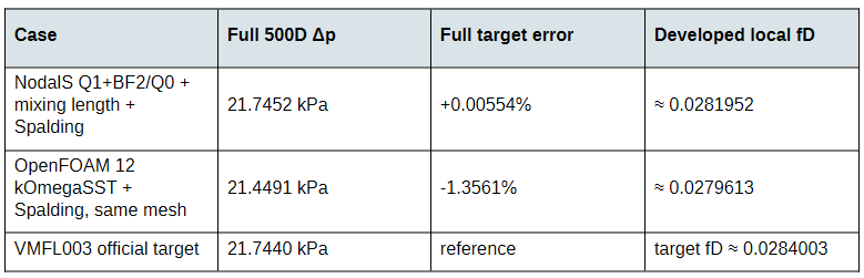
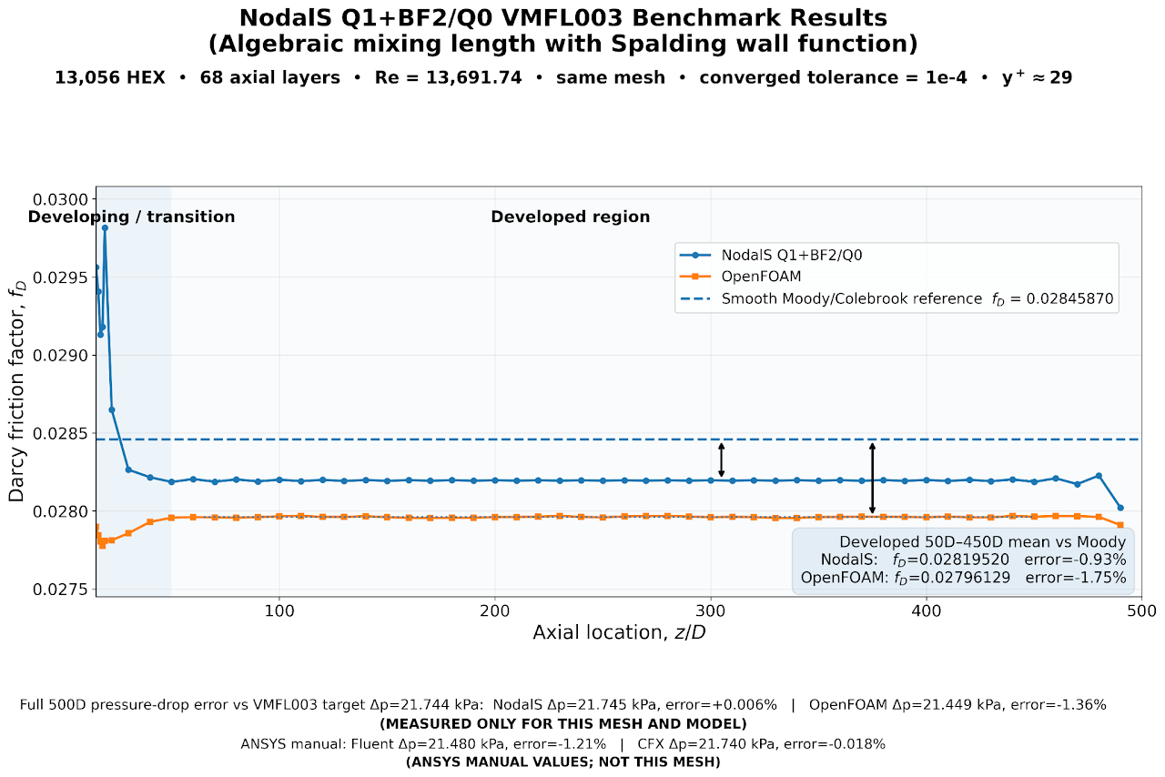
<p class="zfr3Q CDt4Ke " dir="ltr"><span class="C9DxTc ">The eye-catching NodalS full-length result is 21,745.20 Pa, only about +0.0055% from the official 21,744 Pa target. However, this is due to a fortuitous cancellation with the positive inlet error during the flow profile development. A more accurate number the friction factor error in the developed region, roughly 50D to 450D. Here, the NodalS Darcy friction factor was about 0.028195, approximately 0.93% below the smooth Moody/Colebrook value used for the local comparison. </span></p>
<p class="zfr3Q CDt4Ke " dir="ltr"><span class="C9DxTc ">The reason is visible when the pipe is divided into axial zones. The first 50D carries a larger developing/entrance loss, while the long developed portion is slightly under the smooth-pipe friction reference. Over the complete 500D length the two effects almost cancel.</span></p>
</div>
</div>
</div>
</div>
</div>
</div>
</div>
</div>
</div>
</section>
<section id="h.41d9d1b547f2c30b_7" class="yaqOZd">
<div class="mYVXT">
<div class="LS81yb VICjCf j5pSsc db35Fc" tabindex="-1">
<div class="hJDwNd-AhqUyc-OiUrBf Ft7HRd-AhqUyc-OiUrBf purZT-AhqUyc-II5mzb ZcASvf-AhqUyc-II5mzb pSzOP-AhqUyc-qWD73c Ktthjf-AhqUyc-qWD73c JNdkSc SQVYQc yYI8W HQwdzb">
<div class="JNdkSc-SmKAyb LkDMRd">
<div class="">
<div class="oKdM2c ZZyype Kzv0Me">
<div id="h.41d9d1b547f2c30b_4" class="hJDwNd-AhqUyc-OiUrBf Ft7HRd-AhqUyc-OiUrBf jXK9ad D2fZ2 zu5uec OjCsFc dmUFtb">
<div class="jXK9ad-SmKAyb">
<div class="tyJCtd baZpAe">
<div class="t3iYD">
<figure class="CENy8b post__image"><img loading="lazy" role="img" src="https://jade-speculoos-11a861.netlify.app/media/posts/6/24.png" alt="Figure 11: Results of the VMFL003 benchmark for the specific mesh (section 5)" width="1280" height="854" sizes="(max-width: 1920px) 100vw, 1920px" srcset="https://jade-speculoos-11a861.netlify.app/media/posts/6/responsive/24-xs.png 640w ,https://jade-speculoos-11a861.netlify.app/media/posts/6/responsive/24-sm.png 768w ,https://jade-speculoos-11a861.netlify.app/media/posts/6/responsive/24-md.png 1024w ,https://jade-speculoos-11a861.netlify.app/media/posts/6/responsive/24-lg.png 1366w ,https://jade-speculoos-11a861.netlify.app/media/posts/6/responsive/24-xl.png 1600w ,https://jade-speculoos-11a861.netlify.app/media/posts/6/responsive/24-2xl.png 1920w">
<figcaption><span class="C9DxTc ">Figure 11: Results of the VMFL003 benchmark for the specific mesh (section 5)</span></figcaption>
</figure>
</div>
</div>
</div>
</div>
</div>
</div>
</div>
</div>
</div>
</div>
</section>
<section id="h.41d9d1b547f2c30b_13" class="yaqOZd">
<div class="mYVXT">
<div class="LS81yb VICjCf j5pSsc db35Fc" tabindex="-1">
<div class="hJDwNd-AhqUyc-uQSCkd Ft7HRd-AhqUyc-uQSCkd purZT-AhqUyc-II5mzb ZcASvf-AhqUyc-II5mzb pSzOP-AhqUyc-qWD73c Ktthjf-AhqUyc-qWD73c JNdkSc SQVYQc">
<div class="JNdkSc-SmKAyb LkDMRd">
<div class="">
<div class="oKdM2c ZZyype Kzv0Me">
<div id="h.41d9d1b547f2c30b_10" class="hJDwNd-AhqUyc-uQSCkd Ft7HRd-AhqUyc-uQSCkd jXK9ad D2fZ2 zu5uec OjCsFc dmUFtb wHaque g5GTcb">
<div class="jXK9ad-SmKAyb">
<div class="tyJCtd mGzaTb Depvyb baZpAe">
<p class="zfr3Q CDt4Ke " dir="ltr"><span class="C9DxTc ">On the same 13,056-cell mesh, the OpenFOAM 12 comparison used k-omega SST with Spalding-type turbulence wall functions and a strong fixedValue plug inlet. Its full pressure drop was about 21.449 kPa, or -1.36% from the VMFL003 target, and its developed local friction was about 1.75% below the same smooth Moody/Colebrook reference.</span></p>
<p class="zfr3Q CDt4Ke " dir="ltr"><span class="C9DxTc ">This should be read as a same-mesh solver/model comparison, not as a pure discretization comparison. NodalS uses a zero-equation algebraic mixing-length closure and a weak wall traction; OpenFOAM uses transported SST variables, strong no-slip velocity, and its own wall-function machinery.</span></p>
</div>
</div>
</div>
</div>
</div>
</div>
</div>
</div>
</div>
</section>
<section id="h.41d9d1b547f2c30b_17" class="yaqOZd">
<div class="mYVXT">
<div class="LS81yb VICjCf j5pSsc db35Fc" tabindex="-1">
<div class="hJDwNd-AhqUyc-uQSCkd Ft7HRd-AhqUyc-uQSCkd purZT-AhqUyc-II5mzb ZcASvf-AhqUyc-II5mzb pSzOP-AhqUyc-qWD73c Ktthjf-AhqUyc-qWD73c JNdkSc SQVYQc">
<div class="JNdkSc-SmKAyb LkDMRd">
<div class="">
<div class="oKdM2c ZZyype Kzv0Me">
<div id="h.41d9d1b547f2c30b_14" class="hJDwNd-AhqUyc-uQSCkd Ft7HRd-AhqUyc-uQSCkd jXK9ad D2fZ2 zu5uec OjCsFc dmUFtb wHaque g5GTcb">
<div class="jXK9ad-SmKAyb">
<div class="tyJCtd mGzaTb Depvyb baZpAe">
<h2 class="CjVfdc"><span class="C9DxTc ">11. What happened when y+ was changed?</span></h2>
<h3 id="h.q52gmg5m5gca_l" class="zfr3Q OmQG5e CDt4Ke " dir="ltr"></h3>
<p class="zfr3Q CDt4Ke " dir="ltr"><span class="C9DxTc ">An increase in the y+ in the range of 60-100 through a mesh change resulted in a similar result of ~1% error of friction factor for the developed profile. At lower y+ however, the model failure was evident. At lower y+ most meshes did not converge due to high aspect ratio of the hex. Instead the same aspect ratio from the earlier mesh (section 5) was maintained and a 96,768-cell 100D graded mesh was created. This mesh moved the near-wall sampling into roughly y+ = 9-27, with a mean around 17. The nonlinear solution still converged and the downstream friction zones became essentially flat, but the developed Darcy friction rose to about 0.03308: roughly +16.5% relative to the VMFL003 target friction. We were still unable to get OpenFOAM to converge on this mesh even with powerful pressure solver settings.</span></p>
<p class="zfr3Q CDt4Ke " dir="ltr"><span class="C9DxTc ">That behaviour is physically consistent with the limitations of the closure. Near the wall, an undamped Prandtl/Nikuradse mixing length behaves like a log-layer model. Spalding gives a composite relation between mean velocity and wall shear, but it does not automatically correct the separate volume model νt = l²|S| inside the buffer layer.</span></p>
<p class="zfr3Q CDt4Ke " dir="ltr"><span class="C9DxTc ">Further steps for making the model more robust to low y+ would introduce a near-wall damping mechanism such as van Driest damping, or to move to a more complete algebraic model such as Baldwin-Lomax, while keeping the already-tested Q1+BF2/Q0 pressure-velocity architecture unchanged.</span></p>
</div>
</div>
</div>
</div>
</div>
</div>
</div>
</div>
</div>
</section>
<section id="h.41d9d1b547f2c30b_21" class="yaqOZd">
<div class="mYVXT">
<div class="LS81yb VICjCf j5pSsc db35Fc" tabindex="-1">
<div class="hJDwNd-AhqUyc-uQSCkd Ft7HRd-AhqUyc-uQSCkd purZT-AhqUyc-II5mzb ZcASvf-AhqUyc-II5mzb pSzOP-AhqUyc-qWD73c Ktthjf-AhqUyc-qWD73c JNdkSc SQVYQc">
<div class="JNdkSc-SmKAyb LkDMRd">
<div class="">
<div class="oKdM2c ZZyype Kzv0Me">
<div id="h.41d9d1b547f2c30b_18" class="hJDwNd-AhqUyc-uQSCkd Ft7HRd-AhqUyc-uQSCkd jXK9ad D2fZ2 zu5uec OjCsFc dmUFtb wHaque g5GTcb">
<div class="jXK9ad-SmKAyb">
<div class="tyJCtd mGzaTb Depvyb baZpAe">
<h2 class="CjVfdc"><span class="C9DxTc ">12. What this experiment says - and what it does not</span></h2>
<h3 id="h.rz1uhlm9cz10_l" class="zfr3Q OmQG5e CDt4Ke " dir="ltr"></h3>
<ul class="n8H08c UVNKR ">
<li class="zfr3Q TYR86d eD0Rn " dir="ltr">
<p class="zfr3Q CDt4Ke " dir="ltr" role="presentation"><span class="C9DxTc ">A discontinuous constant pressure space can give one integrated continuity equation per cell creating a beneficial cell wise mass conservation </span></p>
</li>
<li class="zfr3Q TYR86d eD0Rn " dir="ltr">
<p class="zfr3Q CDt4Ke " dir="ltr" role="presentation"><span class="C9DxTc ">Shared face-enrichment can make a low-order mixed FE pair pressure-stable without adding PSPG or Rhie-Chow pressure dissipation.</span></p>
</li>
<li class="zfr3Q TYR86d eD0Rn " dir="ltr">
<p class="zfr3Q CDt4Ke " dir="ltr" role="presentation"><span class="C9DxTc ">That topology is compatible with a SIMPLE/SIMPLEC pressure correction based on a cheap diagonal approximation to the momentum inverse.</span></p>
</li>
<li class="zfr3Q TYR86d eD0Rn " dir="ltr">
<p class="zfr3Q CDt4Ke " dir="ltr" role="presentation"><span class="C9DxTc ">The tetrahedral idea transfers naturally to a Q1+BF2/Q0 hexahedral analogue, which is attractive for very long aligned domains.</span></p>
</li>
<li class="zfr3Q TYR86d eD0Rn " dir="ltr">
<p class="zfr3Q CDt4Ke " dir="ltr" role="presentation"><span class="C9DxTc "> Chebyshev-accelerated Jacobi can be a useful low-memory smoother for the tested turbulent pipe, although this is not a universal robustness result.</span></p>
</li>
<li class="zfr3Q TYR86d eD0Rn " dir="ltr">
<p class="zfr3Q CDt4Ke " dir="ltr" role="presentation"><span class="C9DxTc ">A simple algebraic mixing-length closure can give good log-layer results on this benchmark, but it is not a low-y+ turbulence model without additional damping.</span></p>
</li>
</ul>
<p class="zfr3Q CDt4Ke " dir="ltr"><span class="C9DxTc ">The strongest result is therefore not the almost exact full-pipe pressure-drop number by itself. The more interesting result is architectural: a custom mixed finite-element discretization with discontinuous cell pressure and face-enriched continuous velocity can be organized into a familiar segregated SIMPLE workflow, with compact pressure preconditioning and sparse, GPU-friendly linear algebra.</span></p>
<p class="zfr3Q CDt4Ke " dir="ltr"><span class="C9DxTc ">For NodalS, the next interesting questions are broader geometry support, a generic tangential wall formulation, near-wall-damped algebraic turbulence, and eventually transported turbulence and heat-transfer equations. Those extensions can be added without abandoning the central pressure-velocity arrangement.</span></p>
</div>
</div>
</div>
</div>
</div>
</div>
</div>
</div>
</div>
</section>
<section id="h.41d9d1b547f2c30b_25" class="yaqOZd">
<div class="mYVXT">
<div class="LS81yb VICjCf j5pSsc db35Fc" tabindex="-1">
<div class="hJDwNd-AhqUyc-uQSCkd Ft7HRd-AhqUyc-uQSCkd purZT-AhqUyc-II5mzb ZcASvf-AhqUyc-II5mzb pSzOP-AhqUyc-qWD73c Ktthjf-AhqUyc-qWD73c JNdkSc SQVYQc">
<div class="JNdkSc-SmKAyb LkDMRd">
<div class="">
<div class="oKdM2c ZZyype Kzv0Me">
<div id="h.41d9d1b547f2c30b_22" class="hJDwNd-AhqUyc-uQSCkd Ft7HRd-AhqUyc-uQSCkd jXK9ad D2fZ2 zu5uec OjCsFc dmUFtb wHaque g5GTcb">
<div class="jXK9ad-SmKAyb">
<div class="tyJCtd mGzaTb Depvyb baZpAe">
<h2 class="CjVfdc"><span class="C9DxTc ">References and benchmark notes</span></h2>
<h3 id="h.dx5ee55v8xnv_l" class="zfr3Q OmQG5e CDt4Ke " dir="ltr"></h3>
<ol class="n8H08c BKnRcf ">
<li class="zfr3Q TYR86d lsiHE " dir="ltr">
<p class="zfr3Q CDt4Ke " dir="ltr" role="presentation"><span class="C9DxTc ">P. E. Farrell, L. Mitchell and F. Wechsung, “An Augmented Lagrangian Preconditioner for the 3D Stationary Incompressible Navier-Stokes Equations at High Reynolds Number,” arXiv:1810.03315, 2019. The paper discusses the [P1 ⊕ B3^F]^3-P0 face-bubble-enriched pair used as the starting point for the tetrahedral NodalS formulation.</span></p>
</li>
<li class="zfr3Q TYR86d lsiHE " dir="ltr">
<p class="zfr3Q CDt4Ke " dir="ltr" role="presentation"><span class="C9DxTc ">ANSYS Fluid Dynamics Verification Manual, VMFL003: Pressure Drop in Turbulent Flow Through a Pipe. Official target pressure drop used here: 21,744 Pa.</span></p>
</li>
<li class="zfr3Q TYR86d lsiHE " dir="ltr">
<p class="zfr3Q CDt4Ke " dir="ltr" role="presentation"><span class="C9DxTc ">NodalS VMFL003 turbulence benchmark handoff, 3 September 2026. Numerical values, mesh definition, accepted boundary-condition semantics, and low-y+ diagnostics in this article follow the archived benchmark state.</span></p>
</li>
</ol>
<p class="zfr3Q CDt4Ke " dir="ltr"><span class="C9DxTc ">Note on the published comparison: the ANSYS manual Fluent/CFX values use the manual's own model and meshes and are not same-mesh NodalS results. The OpenFOAM comparison described above is the same 13,056-hex topology, but it uses a different turbulence closure and different wall-boundary formulation.</span></p>
</div>
</div>
</div>
</div>
</div>
</div>
</div>
</div>
</div>
</section>
            ]]>
        </content>
    </entry>
    <entry>
        <title>Accelerating Pressure-Based CFD with CUDA and HYPRE AMG</title>
        <author>
            <name>Dr. Jaydeep Deshpande</name>
        </author>
        <link href="https://jade-speculoos-11a861.netlify.app/accelerating-pressure-based-cfd-with-cuda-and-hypre-amg.html"/>
        <id>https://jade-speculoos-11a861.netlify.app/accelerating-pressure-based-cfd-with-cuda-and-hypre-amg.html</id>

        <updated>2026-05-15T10:00:00+05:30</updated>
            <summary type="html">
                <![CDATA[
                    INTRODUCTION Modern GPUs have transformed machine learning and scientific computing by enabling massive computational throughput. Computational Fluid Dynamics (CFD), however, remains one of the more demanding applications because practical engineering simulations often require solving millions of coupled equations over complex geometries. While CPUs have traditionally&hellip;
                ]]>
            </summary>
        <content type="html">
            <![CDATA[
                <section id="h.110085059f6c2f1b_9" class="yaqOZd">
<div class="mYVXT">
<div class="LS81yb VICjCf j5pSsc db35Fc" tabindex="-1">
<div class="hJDwNd-AhqUyc-EehZO Ft7HRd-AhqUyc-EehZO purZT-AhqUyc-II5mzb ZcASvf-AhqUyc-II5mzb pSzOP-AhqUyc-qWD73c Ktthjf-AhqUyc-qWD73c JNdkSc SQVYQc">
<div class="JNdkSc-SmKAyb LkDMRd">
<div class="">
<div class="oKdM2c ZZyype Kzv0Me">
<div id="h.110085059f6c2f1b_12" class="hJDwNd-AhqUyc-EehZO Ft7HRd-AhqUyc-EehZO jXK9ad D2fZ2 zu5uec OjCsFc dmUFtb wHaque g5GTcb">
<div class="jXK9ad-SmKAyb">
<div class="tyJCtd mGzaTb Depvyb baZpAe">
<h2 class="CjVfdc"><span class="C9DxTc ">INTRODUCTION</span></h2>
<h3 id="h.y44msi8uv1r5_l" class="zfr3Q OmQG5e CDt4Ke " dir="ltr"></h3>
<p class="zfr3Q CDt4Ke " dir="ltr"><span class="C9DxTc ">Modern GPUs have transformed machine learning and scientific computing by enabling massive computational throughput. Computational Fluid Dynamics (CFD), however, remains one of the more demanding applications because practical engineering simulations often require solving millions of coupled equations over complex geometries. While CPUs have traditionally been the dominant platform for industrial CFD, modern GPU architectures provide an opportunity to rethink how these simulations are performed. In particular, with recent advances pressure-based incompressible flow solvers have successfully aligned with GPU hardware. This article introduces the development of an educational GPU-accelerated unstructured finite-volume solver built around the SIMPLE and PIMPLE algorithms using CUDA and HYPRE. The objective was not just to create an efficient CFD code, but also to investigate &amp; demonstrate how modern sparse linear algebra and accelerator hardware can unlock new possibilities for pressure-based flow simulation</span></p>
</div>
</div>
</div>
</div>
</div>
</div>
</div>
<div class="hJDwNd-AhqUyc-R6PoUb Ft7HRd-AhqUyc-R6PoUb JNdkSc SQVYQc L6cTce-purZT L6cTce-pSzOP">
<div class="JNdkSc-SmKAyb LkDMRd">
<div class=""> </div>
</div>
</div>
</div>
</div>
</section>
<section id="h.110085059f6c2f1b_181" class="yaqOZd">
<div class="mYVXT">
<div class="LS81yb VICjCf j5pSsc db35Fc" tabindex="-1">
<div class="hJDwNd-AhqUyc-EehZO Ft7HRd-AhqUyc-EehZO purZT-AhqUyc-II5mzb ZcASvf-AhqUyc-II5mzb pSzOP-AhqUyc-qWD73c Ktthjf-AhqUyc-qWD73c JNdkSc SQVYQc">
<div class="JNdkSc-SmKAyb LkDMRd">
<div class="">
<div class="oKdM2c ZZyype Kzv0Me">
<div id="h.110085059f6c2f1b_184" class="hJDwNd-AhqUyc-EehZO Ft7HRd-AhqUyc-EehZO jXK9ad D2fZ2 zu5uec OjCsFc dmUFtb wHaque g5GTcb">
<div class="jXK9ad-SmKAyb">
<div class="tyJCtd mGzaTb Depvyb baZpAe">
<h2 class="CjVfdc"><span class="C9DxTc ">Operator splitting: A practical approximation to the saddle-point Navier Stokes</span></h2>
<h3 id="h.fwmdufbp1ihe_l" class="zfr3Q OmQG5e CDt4Ke " dir="ltr"></h3>
<p class="zfr3Q CDt4Ke " dir="ltr"><span class="C9DxTc ">The starting point for many CFD simulations is the Navier–Stokes equations, which describe conservation of mass and momentum within a fluid. These equations govern a wide range of everyday phenomena, from airflow around vehicles and aircraft to pipe flows, pumps, heat exchangers and environmental transport. In many practical engineering applications the flow speed is much smaller than the speed of sound, meaning density variations become negligible. Under this incompressible assumption, the continuity equation reduces to the simple constraint div(u)=0. While this approximation appears minor, it fundamentally changes the mathematical structure of the problem.</span></p>
</div>
</div>
</div>
</div>
</div>
</div>
</div>
</div>
</div>
</section>
<section id="h.110085059f6c2f1b_188" class="yaqOZd">
<div class="mYVXT">
<div class="LS81yb VICjCf j5pSsc db35Fc" tabindex="-1">
<div class="hJDwNd-AhqUyc-ibL1re Ft7HRd-AhqUyc-ibL1re JNdkSc SQVYQc L6cTce-purZT L6cTce-pSzOP">
<div class="JNdkSc-SmKAyb LkDMRd">
<div class=""> </div>
</div>
</div>
<div class="hJDwNd-AhqUyc-OiUrBf Ft7HRd-AhqUyc-OiUrBf purZT-AhqUyc-II5mzb ZcASvf-AhqUyc-II5mzb pSzOP-AhqUyc-qWD73c Ktthjf-AhqUyc-qWD73c JNdkSc SQVYQc">
<div class="JNdkSc-SmKAyb LkDMRd">
<div class="">
<div class="oKdM2c ZZyype Kzv0Me">
<div id="h.110085059f6c2f1b_185" class="hJDwNd-AhqUyc-OiUrBf Ft7HRd-AhqUyc-OiUrBf jXK9ad D2fZ2 zu5uec OjCsFc dmUFtb wHaque g5GTcb">
<div class="jXK9ad-SmKAyb">
<div class="tyJCtd baZpAe">
<div class="t3iYD"><figure class="CENy8b"><img loading="lazy"  role="img" src="https://lh3.googleusercontent.com/sitesv/AG8ngQWwINzYBh731LGlS0BW2MSVGoohrKWQIy4hCa2tzGaf4oredRHNkGvGL9_G5plAbucHMahpuGD_3IO6CvV4069M2J_C9cP3JynAYtoky7aaqX_jHELfrdODvCJlwb1ZYlnVuUQWOH90A1yh1ZnQ66iZR-1tWIa6spMmJR1Von3f3KengF0irGsLOzcL-PWlCQr76hBFvo0ab9Woz4W8qX1ILgMpNJ_u5-cNRWJb=w1280" data-is-external-image="true"></figure></div>
</div>
</div>
</div>
</div>
</div>
</div>
</div>
</div>
</div>
</section>
<section id="h.110085059f6c2f1b_17" class="yaqOZd">
<div class="mYVXT">
<div class="LS81yb VICjCf j5pSsc db35Fc" tabindex="-1">
<div class="hJDwNd-AhqUyc-EehZO Ft7HRd-AhqUyc-EehZO purZT-AhqUyc-II5mzb ZcASvf-AhqUyc-II5mzb pSzOP-AhqUyc-qWD73c Ktthjf-AhqUyc-qWD73c JNdkSc SQVYQc">
<div class="JNdkSc-SmKAyb LkDMRd">
<div class="">
<div class="oKdM2c ZZyype Kzv0Me">
<div id="h.110085059f6c2f1b_20" class="hJDwNd-AhqUyc-EehZO Ft7HRd-AhqUyc-EehZO jXK9ad D2fZ2 zu5uec OjCsFc dmUFtb wHaque g5GTcb">
<div class="jXK9ad-SmKAyb">
<div class="tyJCtd mGzaTb Depvyb baZpAe">
<p class="zfr3Q CDt4Ke " dir="ltr"><span class="C9DxTc ">Unlike variables such as velocity or temperature, pressure in case of incompressible flows does not possess its own transport equation. Instead, pressure acts as a constraint enforcing incompressibility throughout the domain. In a mathematical sense, pressure behaves as a Lagrange multiplier that ensures the velocity field satisfies continuity. This creates a coupled saddle-point system in which velocity and pressure cannot be solved independently. Directly solving such systems can become computationally demanding, particularly for large three-dimensional industrial meshes.</span></p>
</div>
</div>
</div>
</div>
</div>
</div>
</div>
<div class="hJDwNd-AhqUyc-R6PoUb Ft7HRd-AhqUyc-R6PoUb JNdkSc SQVYQc L6cTce-purZT L6cTce-pSzOP">
<div class="JNdkSc-SmKAyb LkDMRd">
<div class=""> </div>
</div>
</div>
</div>
</div>
</section>
<section id="h.110085059f6c2f1b_192" class="yaqOZd">
<div class="mYVXT">
<div class="LS81yb VICjCf j5pSsc db35Fc" tabindex="-1">
<div class="hJDwNd-AhqUyc-OiUrBf Ft7HRd-AhqUyc-OiUrBf purZT-AhqUyc-II5mzb ZcASvf-AhqUyc-II5mzb pSzOP-AhqUyc-qWD73c Ktthjf-AhqUyc-qWD73c JNdkSc SQVYQc">
<div class="JNdkSc-SmKAyb LkDMRd">
<div class="">
<div class="oKdM2c ZZyype Kzv0Me">
<div id="h.110085059f6c2f1b_189" class="hJDwNd-AhqUyc-OiUrBf Ft7HRd-AhqUyc-OiUrBf jXK9ad D2fZ2 zu5uec OjCsFc dmUFtb wHaque g5GTcb">
<div class="jXK9ad-SmKAyb">
<div class="tyJCtd baZpAe">
<div class="t3iYD"><figure class="CENy8b"><img loading="lazy"  role="img" src="https://lh3.googleusercontent.com/sitesv/AG8ngQVcrOkPbuTprzHt68hQmXozd7IBq9SiUkfAtrLR2oUtnhx76OLU5opqowl9ZuAQ4Gm8dd2LspmlueH7Dc7NPizPcaOui31hXVvWghKm6GjThY5o5QPpADArHqCSiq4_nv74jsjpZICbXyX1f559wnRIPFNAw-dv8_UAqZ35LVWRXlA9IKTVjXQCXCPI-R0jHYyQt1Hd2rduYXX5ZxpqNw2nCElZ7ec2IGeOLLte=w1280" data-is-external-image="true"></figure></div>
</div>
</div>
</div>
</div>
</div>
</div>
</div>
</div>
</div>
</section>
<section id="h.110085059f6c2f1b_25" class="yaqOZd">
<div class="mYVXT">
<div class="LS81yb VICjCf j5pSsc db35Fc" tabindex="-1">
<div class="hJDwNd-AhqUyc-EehZO Ft7HRd-AhqUyc-EehZO purZT-AhqUyc-II5mzb ZcASvf-AhqUyc-II5mzb pSzOP-AhqUyc-qWD73c Ktthjf-AhqUyc-qWD73c JNdkSc SQVYQc">
<div class="JNdkSc-SmKAyb LkDMRd">
<div class="">
<div class="oKdM2c ZZyype Kzv0Me">
<div id="h.110085059f6c2f1b_28" class="hJDwNd-AhqUyc-EehZO Ft7HRd-AhqUyc-EehZO jXK9ad D2fZ2 zu5uec OjCsFc dmUFtb wHaque g5GTcb">
<div class="jXK9ad-SmKAyb">
<div class="tyJCtd mGzaTb Depvyb baZpAe">
<p class="zfr3Q CDt4Ke " dir="ltr"><span class="C9DxTc ">To address this challenge, most practical incompressible flow solvers employ operator splitting methods. Rather than solving velocity and pressure simultaneously as a single monolithic system, the equations are decomposed into smaller and more manageable subproblems. Mathematically this process can be interpreted through a Schur complement factorization of the coupled system. The exact Schur complement operator is expensive to evaluate, but for transient problems and pseudo-transient formulations it can often be approximated using mass matrix information, resulting in efficient split formulations.</span></p>
</div>
</div>
</div>
</div>
</div>
</div>
</div>
</div>
</div>
</section>
<section id="h.110085059f6c2f1b_196" class="yaqOZd">
<div class="mYVXT">
<div class="LS81yb VICjCf j5pSsc db35Fc" tabindex="-1">
<div class="hJDwNd-AhqUyc-ibL1re Ft7HRd-AhqUyc-ibL1re JNdkSc SQVYQc L6cTce-purZT L6cTce-pSzOP">
<div class="JNdkSc-SmKAyb LkDMRd">
<div class=""> </div>
</div>
</div>
<div class="hJDwNd-AhqUyc-OiUrBf Ft7HRd-AhqUyc-OiUrBf purZT-AhqUyc-II5mzb ZcASvf-AhqUyc-II5mzb pSzOP-AhqUyc-qWD73c Ktthjf-AhqUyc-qWD73c JNdkSc SQVYQc">
<div class="JNdkSc-SmKAyb LkDMRd">
<div class="">
<div class="oKdM2c ZZyype Kzv0Me">
<div id="h.110085059f6c2f1b_193" class="hJDwNd-AhqUyc-OiUrBf Ft7HRd-AhqUyc-OiUrBf jXK9ad D2fZ2 zu5uec OjCsFc dmUFtb wHaque g5GTcb">
<div class="jXK9ad-SmKAyb">
<div class="tyJCtd baZpAe">
<div class="t3iYD"><figure class="CENy8b"><img loading="lazy"  role="img" src="https://lh3.googleusercontent.com/sitesv/AG8ngQWeCbdc9uE1fVwSH0weMFGv5WQAqY-E2zdaCikgjSOzYIX9_VQ-eikKAlWLUHi2V8_F16pl7cGoaesoZwPjNVuIEGV9NSXwqpZbeKVFAtXyLLWANWFyrOYsNRJusRJCsaOf_ArF52R6nhWF2IKh3lQd2dvjIMN5eG0wo7u0Fnuxv428JPh-Ydw4YyV4amQAer18RRGo9BfbyL2qIK-AvHoNvqctuQAtWiZop7cgeN4=w1280" data-is-external-image="true"></figure></div>
</div>
</div>
</div>
</div>
</div>
</div>
</div>
</div>
</div>
</section>
<section id="h.110085059f6c2f1b_33" class="yaqOZd">
<div class="mYVXT">
<div class="LS81yb VICjCf j5pSsc db35Fc" tabindex="-1">
<div class="hJDwNd-AhqUyc-EehZO Ft7HRd-AhqUyc-EehZO purZT-AhqUyc-II5mzb ZcASvf-AhqUyc-II5mzb pSzOP-AhqUyc-qWD73c Ktthjf-AhqUyc-qWD73c JNdkSc SQVYQc">
<div class="JNdkSc-SmKAyb LkDMRd">
<div class="">
<div class="oKdM2c ZZyype Kzv0Me">
<div id="h.110085059f6c2f1b_36" class="hJDwNd-AhqUyc-EehZO Ft7HRd-AhqUyc-EehZO jXK9ad D2fZ2 zu5uec OjCsFc dmUFtb wHaque g5GTcb">
<div class="jXK9ad-SmKAyb">
<div class="tyJCtd mGzaTb Depvyb baZpAe">
<p class="zfr3Q CDt4Ke " dir="ltr"><span class="C9DxTc ">This operator split viewpoint naturally leads to predictor-corrector methods. A provisional velocity field is first computed, after which a pressure Poisson equation is solved to enforce continuity. The pressure field is then used to correct both velocity and fluxes. Although this decomposition introduces approximation, it dramatically improves robustness and computational efficiency. The resulting framework forms the foundation of many pressure-based algorithms including SIMPLE, PISO and PIMPLE, which remain among the most widely used approaches in industrial CFD.</span></p>
</div>
</div>
</div>
</div>
</div>
</div>
</div>
</div>
</div>
</section>
<section id="h.110085059f6c2f1b_197" class="yaqOZd">
<div class="mYVXT">
<div class="LS81yb VICjCf j5pSsc db35Fc" tabindex="-1">
<div class="hJDwNd-AhqUyc-EehZO Ft7HRd-AhqUyc-EehZO purZT-AhqUyc-II5mzb ZcASvf-AhqUyc-II5mzb pSzOP-AhqUyc-qWD73c Ktthjf-AhqUyc-qWD73c JNdkSc SQVYQc">
<div class="JNdkSc-SmKAyb LkDMRd">
<div class="">
<div class="oKdM2c ZZyype Kzv0Me">
<div id="h.110085059f6c2f1b_200" class="hJDwNd-AhqUyc-EehZO Ft7HRd-AhqUyc-EehZO jXK9ad D2fZ2 zu5uec OjCsFc dmUFtb wHaque g5GTcb">
<div class="jXK9ad-SmKAyb">
<div class="tyJCtd mGzaTb Depvyb baZpAe">
<h2 class="CjVfdc"><span class="C9DxTc ">The SIMPLE scheme</span></h2>
<h3 id="h.r0sze0npcu75_l" class="zfr3Q OmQG5e CDt4Ke " dir="ltr"></h3>
<p class="zfr3Q CDt4Ke " dir="ltr"><span class="C9DxTc ">Among pressure-based methods, SIMPLE is one of the most important algorithms in industrial CFD. SIMPLE stands for Semi-Implicit Method for Pressure Linked Equations. Its strength is that it converts the coupled incompressible Navier-Stokes problem into a sequence of smaller scalar problems: momentum equations for velocity, followed by a pressure correction equation that enforces mass conservation.</span></p>
<p class="zfr3Q CDt4Ke " dir="ltr"><span class="C9DxTc ">The key idea is simple but powerful. First, the momentum equations are solved using the current pressure field to obtain a predicted velocity. This predicted velocity will generally not satisfy div(u)=0 exactly. Therefore, a pressure correction equation is assembled from the continuity error. Solving this pressure equation gives the correction needed to make the velocity field divergence-free. The pressure, velocity and face fluxes are then updated, and the process is repeated until both the velocity change and continuity residual become small.</span></p>
<p class="zfr3Q CDt4Ke " dir="ltr"><span class="C9DxTc ">SIMPLE remains extremely useful in practical CFD: it avoids solving the full saddle-point system directly, while still preserving the pressure-velocity coupling needed for incompressible flow. It is robust, modular and works well with complex unstructured finite-volume meshes. It also maps well to modern CFD software design because the velocity equations behave like scalar transport equations, while the pressure correction equation behaves like a Poisson-type elliptic solve. In the GPU solver developed here.</span></p>
</div>
</div>
</div>
</div>
</div>
</div>
</div>
</div>
</div>
</section>
<section id="h.110085059f6c2f1b_201" class="yaqOZd">
<div class="mYVXT">
<div class="LS81yb VICjCf j5pSsc db35Fc" tabindex="-1">
<div class="hJDwNd-AhqUyc-EehZO Ft7HRd-AhqUyc-EehZO purZT-AhqUyc-II5mzb ZcASvf-AhqUyc-II5mzb pSzOP-AhqUyc-qWD73c Ktthjf-AhqUyc-qWD73c JNdkSc SQVYQc">
<div class="JNdkSc-SmKAyb LkDMRd">
<div class="">
<div class="oKdM2c ZZyype Kzv0Me">
<div id="h.110085059f6c2f1b_204" class="hJDwNd-AhqUyc-EehZO Ft7HRd-AhqUyc-EehZO jXK9ad D2fZ2 zu5uec OjCsFc dmUFtb wHaque g5GTcb">
<div class="jXK9ad-SmKAyb">
<div class="tyJCtd mGzaTb Depvyb baZpAe">
<p class="zfr3Q CDt4Ke " dir="ltr"><span class="C9DxTc ">SIMPLE loop used in the GPU solver</span></p>
<p class="zfr3Q CDt4Ke " dir="ltr"><span class="C9DxTc ">----------------------------------</span></p>
<br>
<p class="zfr3Q CDt4Ke " dir="ltr"><span class="C9DxTc ">Start with U, p and phi</span></p>
<br>
<p class="zfr3Q CDt4Ke " dir="ltr"><span class="C9DxTc ">        |</span></p>
<p class="zfr3Q CDt4Ke " dir="ltr"><span class="C9DxTc ">        v</span></p>
<br>
<p class="zfr3Q CDt4Ke " dir="ltr"><span class="C9DxTc ">Compute grad(p)</span></p>
<br>
<p class="zfr3Q CDt4Ke " dir="ltr"><span class="C9DxTc ">        |</span></p>
<p class="zfr3Q CDt4Ke " dir="ltr"><span class="C9DxTc ">        v</span></p>
<br>
<p class="zfr3Q CDt4Ke " dir="ltr"><span class="C9DxTc ">Solve momentum equations using current pressure</span></p>
<p class="zfr3Q CDt4Ke " dir="ltr"><span class="C9DxTc ">-----------------------------------------------</span></p>
<p class="zfr3Q CDt4Ke " dir="ltr"><span class="C9DxTc ">A(U) U* = H - grad(p)</span></p>
<br>
<p class="zfr3Q CDt4Ke " dir="ltr"><span class="C9DxTc ">Result:</span></p>
<p class="zfr3Q CDt4Ke " dir="ltr"><span class="C9DxTc ">    U* = predicted cell-centered velocity</span></p>
<br>
<p class="zfr3Q CDt4Ke " dir="ltr"><span class="C9DxTc ">        |</span></p>
<p class="zfr3Q CDt4Ke " dir="ltr"><span class="C9DxTc ">        v</span></p>
<br>
<p class="zfr3Q CDt4Ke " dir="ltr"><span class="C9DxTc ">Extract rAU from the momentum operator</span></p>
<p class="zfr3Q CDt4Ke " dir="ltr"><span class="C9DxTc ">--------------------------------------</span></p>
<p class="zfr3Q CDt4Ke " dir="ltr"><span class="C9DxTc ">rAU tells how strongly pressure correction changes velocity</span></p>
<br>
<p class="zfr3Q CDt4Ke " dir="ltr"><span class="C9DxTc ">        |</span></p>
<p class="zfr3Q CDt4Ke " dir="ltr"><span class="C9DxTc ">        v</span></p>
<br>
<p class="zfr3Q CDt4Ke " dir="ltr"><span class="C9DxTc ">Build pressure-correction matrix</span></p>
<p class="zfr3Q CDt4Ke " dir="ltr"><span class="C9DxTc ">--------------------------------</span></p>
<p class="zfr3Q CDt4Ke " dir="ltr"><span class="C9DxTc ">The pressure equation uses rAU as its main coefficient</span></p>
<br>
<p class="zfr3Q CDt4Ke " dir="ltr"><span class="C9DxTc ">        |</span></p>
<p class="zfr3Q CDt4Ke " dir="ltr"><span class="C9DxTc ">        v</span></p>
<br>
<p class="zfr3Q CDt4Ke " dir="ltr"><span class="C9DxTc ">Construct predicted face flux</span></p>
<p class="zfr3Q CDt4Ke " dir="ltr"><span class="C9DxTc ">-----------------------------</span></p>
<p class="zfr3Q CDt4Ke " dir="ltr"><span class="C9DxTc ">phiStar = pressure-coupled face flux from the momentum predictor</span></p>
<br>
<p class="zfr3Q CDt4Ke " dir="ltr"><span class="C9DxTc ">Rhie-Chow interpolation is used here to avoid pressure-velocity decoupling</span></p>
<p class="zfr3Q CDt4Ke " dir="ltr"><span class="C9DxTc ">on the collocated finite-volume mesh.</span></p>
<br>
<p class="zfr3Q CDt4Ke " dir="ltr"><span class="C9DxTc ">        |</span></p>
<p class="zfr3Q CDt4Ke " dir="ltr"><span class="C9DxTc ">        v</span></p>
<br>
<p class="zfr3Q CDt4Ke " dir="ltr"><span class="C9DxTc ">Compute continuity error</span></p>
<p class="zfr3Q CDt4Ke " dir="ltr"><span class="C9DxTc ">------------------------</span></p>
<p class="zfr3Q CDt4Ke " dir="ltr"><span class="C9DxTc ">continuity error = div(phiStar)</span></p>
<br>
<p class="zfr3Q CDt4Ke " dir="ltr"><span class="C9DxTc ">        |</span></p>
<p class="zfr3Q CDt4Ke " dir="ltr"><span class="C9DxTc ">        v</span></p>
<br>
<p class="zfr3Q CDt4Ke " dir="ltr"><span class="C9DxTc ">Solve pressure correction equation</span></p>
<p class="zfr3Q CDt4Ke " dir="ltr"><span class="C9DxTc ">----------------------------------</span></p>
<p class="zfr3Q CDt4Ke " dir="ltr"><span class="C9DxTc ">Find the pressure correction needed to remove the continuity error</span></p>
<br>
<p class="zfr3Q CDt4Ke " dir="ltr"><span class="C9DxTc ">        |</span></p>
<p class="zfr3Q CDt4Ke " dir="ltr"><span class="C9DxTc ">        v</span></p>
<br>
<p class="zfr3Q CDt4Ke " dir="ltr"><span class="C9DxTc ">Correct face flux</span></p>
<p class="zfr3Q CDt4Ke " dir="ltr"><span class="C9DxTc ">-----------------</span></p>
<p class="zfr3Q CDt4Ke " dir="ltr"><span class="C9DxTc ">phi = phiStar - pressure correction flux</span></p>
<br>
<p class="zfr3Q CDt4Ke " dir="ltr"><span class="C9DxTc ">This gives the conservative finite-volume flux.</span></p>
<br>
<p class="zfr3Q CDt4Ke " dir="ltr"><span class="C9DxTc ">        |</span></p>
<p class="zfr3Q CDt4Ke " dir="ltr"><span class="C9DxTc ">        v</span></p>
<br>
<p class="zfr3Q CDt4Ke " dir="ltr"><span class="C9DxTc ">Update pressure</span></p>
<p class="zfr3Q CDt4Ke " dir="ltr"><span class="C9DxTc ">---------------</span></p>
<p class="zfr3Q CDt4Ke " dir="ltr"><span class="C9DxTc ">p = p + relaxed pressure correction</span></p>
<br>
<p class="zfr3Q CDt4Ke " dir="ltr"><span class="C9DxTc ">        |</span></p>
<p class="zfr3Q CDt4Ke " dir="ltr"><span class="C9DxTc ">        v</span></p>
<br>
<p class="zfr3Q CDt4Ke " dir="ltr"><span class="C9DxTc ">Correct cell-centered velocity</span></p>
<p class="zfr3Q CDt4Ke " dir="ltr"><span class="C9DxTc ">------------------------------</span></p>
<p class="zfr3Q CDt4Ke " dir="ltr"><span class="C9DxTc ">U = U* - rAU grad(pressure correction)</span></p>
<br>
<p class="zfr3Q CDt4Ke " dir="ltr"><span class="C9DxTc ">        |</span></p>
<p class="zfr3Q CDt4Ke " dir="ltr"><span class="C9DxTc ">        v</span></p>
<br>
<p class="zfr3Q CDt4Ke " dir="ltr"><span class="C9DxTc ">Check convergence</span></p>
<p class="zfr3Q CDt4Ke " dir="ltr"><span class="C9DxTc ">-----------------</span></p>
<p class="zfr3Q CDt4Ke " dir="ltr"><span class="C9DxTc ">Is div(phi) small?</span></p>
<p class="zfr3Q CDt4Ke " dir="ltr"><span class="C9DxTc ">Is the velocity change small?</span></p>
<br>
<p class="zfr3Q CDt4Ke " dir="ltr"><span class="C9DxTc ">        |</span></p>
<p class="zfr3Q CDt4Ke " dir="ltr"><span class="C9DxTc ">        v</span></p>
<br>
<p class="zfr3Q CDt4Ke " dir="ltr"><span class="C9DxTc ">If not converged:</span></p>
<p class="zfr3Q CDt4Ke " dir="ltr"><span class="C9DxTc ">    repeat SIMPLE loop</span></p>
<br>
<p class="zfr3Q CDt4Ke " dir="ltr"><span class="C9DxTc ">If converged:</span></p>
<p class="zfr3Q CDt4Ke " dir="ltr"><span class="C9DxTc ">    write fields and postprocess quantities such as drag and lift</span></p>
</div>
</div>
</div>
</div>
</div>
</div>
</div>
<div class="hJDwNd-AhqUyc-R6PoUb Ft7HRd-AhqUyc-R6PoUb JNdkSc SQVYQc L6cTce-purZT L6cTce-pSzOP">
<div class="JNdkSc-SmKAyb LkDMRd"> </div>
</div>
</div>
</div>
</section>
<section id="h.110085059f6c2f1b_49" class="yaqOZd">
<div class="mYVXT">
<div class="LS81yb VICjCf j5pSsc db35Fc" tabindex="-1">
<div class="hJDwNd-AhqUyc-R6PoUb Ft7HRd-AhqUyc-R6PoUb JNdkSc SQVYQc L6cTce-purZT L6cTce-pSzOP">
<div class="JNdkSc-SmKAyb LkDMRd">
<div class=""> </div>
</div>
</div>
<div class="hJDwNd-AhqUyc-EehZO Ft7HRd-AhqUyc-EehZO purZT-AhqUyc-II5mzb ZcASvf-AhqUyc-II5mzb pSzOP-AhqUyc-qWD73c Ktthjf-AhqUyc-qWD73c JNdkSc SQVYQc">
<div class="JNdkSc-SmKAyb LkDMRd">
<div class="">
<div class="oKdM2c ZZyype Kzv0Me">
<div id="h.110085059f6c2f1b_52" class="hJDwNd-AhqUyc-EehZO Ft7HRd-AhqUyc-EehZO jXK9ad D2fZ2 zu5uec OjCsFc dmUFtb wHaque g5GTcb">
<div class="jXK9ad-SmKAyb">
<div class="tyJCtd mGzaTb Depvyb baZpAe">
<p class="zfr3Q CDt4Ke " dir="ltr"><span class="C9DxTc ">SIMPLE starts by solving the momentum equations using the current pressure field. This produces an intermediate cell-centered velocity field, usually called U*. However, this predicted velocity field is not guaranteed to satisfy incompressibility. In other words, the face fluxes constructed from the momentum predictor may not balance exactly across each control volume.</span></p>
<p class="zfr3Q CDt4Ke " dir="ltr"><span class="C9DxTc ">The next step is therefore to measure this mass imbalance and use it to build a pressure correction equation. This pressure correction equation determines how the pressure field must change in order to remove the continuity error. After this equation is solved, the solver corrects the face fluxes, updates the pressure field, and corrects the cell-centered velocity field. The corrected face flux ensures finite-volume mass conservation, while the corrected velocity field becomes the starting point for the next momentum solve.</span></p>
<p class="zfr3Q CDt4Ke " dir="ltr"><span class="C9DxTc ">This process is repeated until the continuity error and the velocity change become sufficiently small. In this way, SIMPLE avoids solving the full coupled velocity-pressure saddle-point system directly. Instead, it converts the incompressible flow problem into a sequence of more manageable momentum solves and pressure correction solves.</span></p>
<p class="zfr3Q CDt4Ke " dir="ltr"><span class="C9DxTc ">Two details are especially important in making this procedure work well. The first is rAU, the inverse of the diagonal coefficient of the momentum equation. This quantity tells the solver how strongly a pressure correction changes the velocity field. In the pressure correction equation, rAU plays a role similar to a diffusion coefficient because it controls how the pressure correction propagates through the mesh to remove mass imbalance.</span></p>
<p class="zfr3Q CDt4Ke " dir="ltr"><span class="C9DxTc ">The second important detail is Rhie-Chow interpolation. In a collocated finite-volume method, pressure and velocity are both stored at cell centers. If the face flux is obtained only by simple interpolation of cell-centered velocity, pressure and velocity can decouple, leading to non-physical checkerboard pressure patterns. Rhie-Chow interpolation avoids this by constructing the face flux in a pressure-sensitive way. SIMPLE corrects phi directly because finite-volume conservation is enforced through face fluxes, while the corrected cell-centered velocity keeps the stored velocity field consistent for the next iteration.</span></p>
</div>
</div>
</div>
</div>
</div>
</div>
</div>
<div class="hJDwNd-AhqUyc-R6PoUb Ft7HRd-AhqUyc-R6PoUb JNdkSc SQVYQc L6cTce-purZT L6cTce-pSzOP">
<div class="JNdkSc-SmKAyb LkDMRd"> </div>
</div>
</div>
</div>
</section>
<section id="h.110085059f6c2f1b_57" class="yaqOZd">
<div class="mYVXT">
<div class="LS81yb VICjCf j5pSsc db35Fc" tabindex="-1">
<div class="hJDwNd-AhqUyc-EehZO Ft7HRd-AhqUyc-EehZO purZT-AhqUyc-II5mzb ZcASvf-AhqUyc-II5mzb pSzOP-AhqUyc-qWD73c Ktthjf-AhqUyc-qWD73c JNdkSc SQVYQc">
<div class="JNdkSc-SmKAyb LkDMRd">
<div class="">
<div class="oKdM2c ZZyype Kzv0Me">
<div id="h.110085059f6c2f1b_60" class="hJDwNd-AhqUyc-EehZO Ft7HRd-AhqUyc-EehZO jXK9ad D2fZ2 zu5uec OjCsFc dmUFtb wHaque g5GTcb">
<div class="jXK9ad-SmKAyb">
<div class="tyJCtd mGzaTb Depvyb baZpAe">
<div class="PPhIP rviiZ"> </div>
<h2 class="CjVfdc"><span class="C9DxTc ">AMG: Solving the Pressure Poisson within practical timelines </span></h2>
<h3 id="h.brk3un2dk4pi_l" class="zfr3Q OmQG5e CDt4Ke " dir="ltr"></h3>
<p class="zfr3Q CDt4Ke " dir="ltr"><span class="C9DxTc ">The pressure correction equation that appears in incompressible flow solvers is Poisson-like. This is one reason pressure-based CFD is computationally demanding. A Poisson equation is elliptic, which means information is coupled globally across the domain. A local correction in one region can influence the pressure field everywhere else. As a result, the pressure solve is often the most expensive part of a SIMPLE or PIMPLE iteration.</span></p>
</div>
</div>
</div>
</div>
</div>
</div>
</div>
<div class="hJDwNd-AhqUyc-R6PoUb Ft7HRd-AhqUyc-R6PoUb JNdkSc SQVYQc L6cTce-purZT L6cTce-pSzOP">
<div class="JNdkSc-SmKAyb LkDMRd">
<div class=""> </div>
</div>
</div>
</div>
</div>
</section>
<section id="h.110085059f6c2f1b_208" class="yaqOZd">
<div class="mYVXT">
<div class="LS81yb VICjCf j5pSsc db35Fc" tabindex="-1">
<div class="hJDwNd-AhqUyc-OiUrBf Ft7HRd-AhqUyc-OiUrBf purZT-AhqUyc-II5mzb ZcASvf-AhqUyc-II5mzb pSzOP-AhqUyc-qWD73c Ktthjf-AhqUyc-qWD73c JNdkSc SQVYQc">
<div class="JNdkSc-SmKAyb LkDMRd">
<div class="">
<div class="oKdM2c ZZyype Kzv0Me">
<div id="h.110085059f6c2f1b_205" class="hJDwNd-AhqUyc-OiUrBf Ft7HRd-AhqUyc-OiUrBf jXK9ad D2fZ2 zu5uec OjCsFc dmUFtb wHaque g5GTcb">
<div class="jXK9ad-SmKAyb">
<div class="tyJCtd baZpAe">
<div class="t3iYD"><figure class="CENy8b"><img loading="lazy"  role="img" src="https://lh3.googleusercontent.com/sitesv/AG8ngQWbY2ECQMRXbhXVnX7CihscfNSdCkyT7OVIuTVSNhB8oq3eQzr75LTt3UekTf_lzsEoVS7W1Pf5gWjuEpR9nBq6RsIE4sjJNsv-n0Ejgaf-1Wge00KmZo0glVOJgNJynnYjRsD1_SV1D324O94ZJTgqpUxUrglVbUzMiKQp8h7NzxueUi3YstPMG9iOPUErNuO7zSjXeoX12bmCsoQzSSgegKFZ25GCKQhB6FWg=w1280" data-is-external-image="true"></figure></div>
</div>
</div>
</div>
</div>
</div>
</div>
</div>
</div>
</div>
</section>
<section id="h.110085059f6c2f1b_65" class="yaqOZd">
<div class="mYVXT">
<div class="LS81yb VICjCf j5pSsc db35Fc" tabindex="-1">
<div class="hJDwNd-AhqUyc-EehZO Ft7HRd-AhqUyc-EehZO purZT-AhqUyc-II5mzb ZcASvf-AhqUyc-II5mzb pSzOP-AhqUyc-qWD73c Ktthjf-AhqUyc-qWD73c JNdkSc SQVYQc">
<div class="JNdkSc-SmKAyb LkDMRd">
<div class="">
<div class="oKdM2c ZZyype Kzv0Me">
<div id="h.110085059f6c2f1b_68" class="hJDwNd-AhqUyc-EehZO Ft7HRd-AhqUyc-EehZO jXK9ad D2fZ2 zu5uec OjCsFc dmUFtb wHaque g5GTcb">
<div class="jXK9ad-SmKAyb">
<div class="tyJCtd mGzaTb Depvyb baZpAe">
<p class="zfr3Q CDt4Ke " dir="ltr"><span class="C9DxTc ">A useful way to understand this is through the heat equation. If the heat equation is written in terms of Fourier modes, each mode decays at a rate proportional to D k^2, where D is the diffusion coefficient and k is the wave number. High-frequency oscillations have large k, so they decay rapidly. Long-wavelength oscillations have small k, so they decay much more slowly.</span></p>
<p class="zfr3Q CDt4Ke " dir="ltr"><span class="C9DxTc ">This same idea is central to multigrid methods. Basic iterative smoothers are very good at removing high-frequency error, but they are much less effective at removing smooth, long-wavelength error. Multigrid solves this problem by transferring the error to coarser grids. On a coarse grid, what looked like a long-wavelength error on the fine grid becomes easier to represent and remove. By moving between fine and coarse levels, multigrid can reduce error across many length scales very efficiently.</span></p>
<p class="zfr3Q CDt4Ke " dir="ltr"><span class="C9DxTc ">In geometric multigrid, these coarse levels are created from actual coarse meshes or structured grid hierarchies. This can be extremely effective, but it is not always convenient for complex unstructured industrial meshes. Creating high-quality coarse grids and transfer operators can become difficult, especially when the mesh contains arbitrary polyhedra, local refinement or complicated geometry.</span></p>
<p class="zfr3Q CDt4Ke " dir="ltr"><span class="C9DxTc ">Algebraic multigrid addresses this problem differently. Instead of requiring explicit geometric coarse grids, AMG builds the multigrid hierarchy from the sparse matrix itself. The matrix contains information about which unknowns are strongly coupled, and AMG uses this algebraic structure to form coarse levels, interpolation operators and smoothers. This makes AMG especially attractive for unstructured finite-volume CFD, where the pressure equation is naturally represented as a sparse matrix.</span></p>
<p class="zfr3Q CDt4Ke " dir="ltr"><span class="C9DxTc ">This is also where GPUs become important. AMG is computationally heavy: it involves sparse matrix-vector products, smoothing operations, residual calculations, restriction, interpolation and coarse-grid corrections. These operations have large throughput requirements and are repeated many times during a pressure solve. Modern GPUs can be designed exactly for this kind of high-throughput parallel work; and therefore, a pressure-based CFD solver can benefit strongly when its pressure correction equation is solved using a GPU-capable AMG library.</span></p>
<p class="zfr3Q CDt4Ke " dir="ltr"><span class="C9DxTc ">Several GPU-oriented sparse linear algebra and AMG libraries exist, including HYPRE/BoomerAMG, NVIDIA AmgX, PETSc with GPU backends, Trilinos/MueLu and Ginkgo. In this solver, HYPRE was chosen because it provides a mature parallel sparse linear solvers and the well-optimized BoomerAMG algebraic multigrid preconditioner. The pressure correction equation is solved using a Krylov method accelerated by BoomerAMG, while the surrounding finite-volume assembly and correction operations are kept on the GPU. This combination allows the solver to preserve the robustness of pressure-based CFD while taking advantage of modern GPU throughput.</span></p>
</div>
</div>
</div>
</div>
</div>
</div>
</div>
</div>
</div>
</section>
<section id="h.110085059f6c2f1b_69" class="yaqOZd">
<div class="mYVXT">
<div class="LS81yb VICjCf j5pSsc db35Fc" tabindex="-1">
<div class="hJDwNd-AhqUyc-EehZO Ft7HRd-AhqUyc-EehZO purZT-AhqUyc-II5mzb ZcASvf-AhqUyc-II5mzb pSzOP-AhqUyc-qWD73c Ktthjf-AhqUyc-qWD73c JNdkSc SQVYQc">
<div class="JNdkSc-SmKAyb LkDMRd">
<div class="">
<div class="oKdM2c ZZyype Kzv0Me">
<div id="h.110085059f6c2f1b_72" class="hJDwNd-AhqUyc-EehZO Ft7HRd-AhqUyc-EehZO jXK9ad D2fZ2 zu5uec OjCsFc dmUFtb wHaque g5GTcb">
<div class="jXK9ad-SmKAyb">
<div class="tyJCtd mGzaTb Depvyb baZpAe">
<h2 class="CjVfdc"><span class="C9DxTc ">The code structure:</span></h2>
<h3 id="h.4a3si3bd44zg_l" class="zfr3Q OmQG5e CDt4Ke " dir="ltr"></h3>
<p class="zfr3Q CDt4Ke " dir="ltr"><span class="C9DxTc ">The code is organized around keeping the finite-volume physics modular, and keeping the expensive numerical work on the GPU. The solver reads an OpenFOAM polyMesh, applies boundary conditions from runtime case files, assembles the finite-volume equations, and solves the resulting sparse systems using CUDA and HYPRE.</span></p>
<p class="zfr3Q CDt4Ke " dir="ltr"><span class="C9DxTc ">At the top level, the code contains a main flow solver application and a set of reusable numerical libraries. A simplified view of the structure is:</span></p>
<p class="zfr3Q CDt4Ke " dir="ltr"><span class="C9DxTc ">    anabasis </span><a class="XqQF9c" href="https://github.com/JD63021/Anabasis" target="_blank" rel="noopener"><span class="C9DxTc aw5Odc ">(link to the github repo)</span></a></p>
<p class="zfr3Q CDt4Ke " dir="ltr"><span class="C9DxTc ">        |</span></p>
<p class="zfr3Q CDt4Ke " dir="ltr"><span class="C9DxTc ">        |-- apps/simple_gpu</span></p>
<p class="zfr3Q CDt4Ke " dir="ltr"><span class="C9DxTc ">        |       |</span></p>
<p class="zfr3Q CDt4Ke " dir="ltr"><span class="C9DxTc ">        |       |-- main.cu</span></p>
<p class="zfr3Q CDt4Ke " dir="ltr"><span class="C9DxTc ">        |       |-- boundary condition handling</span></p>
<p class="zfr3Q CDt4Ke " dir="ltr"><span class="C9DxTc ">        |       |-- patch geometry</span></p>
<p class="zfr3Q CDt4Ke " dir="ltr"><span class="C9DxTc ">        |       |-- velocity boundary evaluation</span></p>
<p class="zfr3Q CDt4Ke " dir="ltr"><span class="C9DxTc ">        |</span></p>
<p class="zfr3Q CDt4Ke " dir="ltr"><span class="C9DxTc ">        |-- libpoisson</span></p>
<p class="zfr3Q CDt4Ke " dir="ltr"><span class="C9DxTc ">        |       |</span></p>
<p class="zfr3Q CDt4Ke " dir="ltr"><span class="C9DxTc ">        |       |-- mesh utilities</span></p>
<p class="zfr3Q CDt4Ke " dir="ltr"><span class="C9DxTc ">        |       |-- gradient reconstruction</span></p>
<p class="zfr3Q CDt4Ke " dir="ltr"><span class="C9DxTc ">        |       |-- scalar elliptic / Poisson utilities</span></p>
<p class="zfr3Q CDt4Ke " dir="ltr"><span class="C9DxTc ">        |       |-- HYPRE backend</span></p>
<p class="zfr3Q CDt4Ke " dir="ltr"><span class="C9DxTc ">        |</span></p>
<p class="zfr3Q CDt4Ke " dir="ltr"><span class="C9DxTc ">        |-- libscalar</span></p>
<p class="zfr3Q CDt4Ke " dir="ltr"><span class="C9DxTc ">        |       |</span></p>
<p class="zfr3Q CDt4Ke " dir="ltr"><span class="C9DxTc ">        |       |-- scalar transport solver</span></p>
<p class="zfr3Q CDt4Ke " dir="ltr"><span class="C9DxTc ">        |       |-- convection and diffusion operators</span></p>
<p class="zfr3Q CDt4Ke " dir="ltr"><span class="C9DxTc ">        |       |-- scalar boundary conditions</span></p>
<p class="zfr3Q CDt4Ke " dir="ltr"><span class="C9DxTc ">        |</span></p>
<p class="zfr3Q CDt4Ke " dir="ltr"><span class="C9DxTc ">        |-- cases</span></p>
<p class="zfr3Q CDt4Ke " dir="ltr"><span class="C9DxTc ">        |       |</span></p>
<p class="zfr3Q CDt4Ke " dir="ltr"><span class="C9DxTc ">        |       |-- reference case files</span></p>
<p class="zfr3Q CDt4Ke " dir="ltr"><span class="C9DxTc ">        |</span></p>
<p class="zfr3Q CDt4Ke " dir="ltr"><span class="C9DxTc ">        |-- docs</span></p>
<p class="zfr3Q CDt4Ke " dir="ltr"><span class="C9DxTc ">                |</span></p>
<p class="zfr3Q CDt4Ke " dir="ltr"><span class="C9DxTc ">                |-- build and run notes</span></p>
<br>
<p class="zfr3Q CDt4Ke " dir="ltr"><span class="C9DxTc ">The scalar transport library is important because many CFD equations have a similar finite-volume structure. Passive scalar transport, temperature, species concentration, turbulence kinetic energy and dissipation can all be written in convection-diffusion-source form. This makes the scalar transport module a natural path toward additional physics such as heat transfer, species transport, level-set equations and RANS turbulence models.</span></p>
<p class="zfr3Q CDt4Ke " dir="ltr"><span class="C9DxTc ">In simplified form, these scalar equations look like:</span></p>
<p class="zfr3Q CDt4Ke " dir="ltr"><span class="C9DxTc ">    convection of phi</span></p>
<p class="zfr3Q CDt4Ke " dir="ltr"><span class="C9DxTc ">  + diffusion of phi</span></p>
<p class="zfr3Q CDt4Ke " dir="ltr"><span class="C9DxTc ">  + source terms</span></p>
<p class="zfr3Q CDt4Ke " dir="ltr"><span class="C9DxTc ">  = 0</span></p>
<br>
<p class="zfr3Q CDt4Ke " dir="ltr"><span class="C9DxTc ">The GPU execution flow can be summarized as:</span></p>
<br>
<p class="zfr3Q CDt4Ke " dir="ltr"><span class="C9DxTc ">    CUDA kernel:</span></p>
<p class="zfr3Q CDt4Ke " dir="ltr"><span class="C9DxTc ">        assemble momentum matrices and right-hand sides</span></p>
<br>
<p class="zfr3Q CDt4Ke " dir="ltr"><span class="C9DxTc ">    HYPRE:</span></p>
<p class="zfr3Q CDt4Ke " dir="ltr"><span class="C9DxTc ">        solve momentum systems</span></p>
<br>
<p class="zfr3Q CDt4Ke " dir="ltr"><span class="C9DxTc ">    CUDA kernel:</span></p>
<p class="zfr3Q CDt4Ke " dir="ltr"><span class="C9DxTc ">        extract rAU from the momentum operator</span></p>
<br>
<p class="zfr3Q CDt4Ke " dir="ltr"><span class="C9DxTc ">    CUDA kernel:</span></p>
<p class="zfr3Q CDt4Ke " dir="ltr"><span class="C9DxTc ">        construct pressure-coupled face fluxes</span></p>
<br>
<p class="zfr3Q CDt4Ke " dir="ltr"><span class="C9DxTc ">    CUDA kernel:</span></p>
<p class="zfr3Q CDt4Ke " dir="ltr"><span class="C9DxTc ">        build pressure correction right-hand side</span></p>
<br>
<p class="zfr3Q CDt4Ke " dir="ltr"><span class="C9DxTc ">    HYPRE:</span></p>
<p class="zfr3Q CDt4Ke " dir="ltr"><span class="C9DxTc ">        solve pressure correction system using PCG + AMG</span></p>
<br>
<p class="zfr3Q CDt4Ke " dir="ltr"><span class="C9DxTc ">    CUDA kernel:</span></p>
<p class="zfr3Q CDt4Ke " dir="ltr"><span class="C9DxTc ">        correct face fluxes</span></p>
<br>
<p class="zfr3Q CDt4Ke " dir="ltr"><span class="C9DxTc ">    CUDA kernel:</span></p>
<p class="zfr3Q CDt4Ke " dir="ltr"><span class="C9DxTc ">        update pressure and velocity</span></p>
<br>
<p class="zfr3Q CDt4Ke " dir="ltr"><span class="C9DxTc ">    CUDA kernel:</span></p>
<p class="zfr3Q CDt4Ke " dir="ltr"><span class="C9DxTc ">        compute residuals and convergence measures</span></p>
<br>
<p class="zfr3Q CDt4Ke " dir="ltr"><span class="C9DxTc ">The important performance choice is to avoid repeatedly moving large CFD fields between CPU and GPU. Once the mesh and fields are on the device, the major assembly, correction and residual operations remain GPU-resident. This is essential because realistic unstructured CFD cases contain millions of cells and faces. Repeated CPU-GPU transfers would quickly destroy the benefit of acceleration.</span></p>
<p class="zfr3Q CDt4Ke " dir="ltr"><span class="C9DxTc ">The same structure also extends naturally from SIMPLE to PIMPLE. SIMPLE is mainly used for steady-state problems, while PIMPLE places a similar pressure-velocity correction process inside a transient time-stepping loop. This allows the solver to use the robustness of SIMPLE while moving toward unsteady incompressible simulations. From a software point of view, the same core operations remain central: momentum prediction, pressure correction, flux correction and velocity correction.</span></p>
<p class="zfr3Q CDt4Ke " dir="ltr"><span class="C9DxTc ">In summary the GPU CFD framework is as follows: (1) The scalar transport module providing a route to additional equations and turbulence models. (2) The pressure solver machinery provides the core incompressible flow capability. (3) HYPRE supplies AMG-accelerated sparse linear algebra. CUDA kernels keep the finite-volume operations close to the data. Together, these pieces form the foundation of a pressure-based unstructured finite-volume solver designed for modern GPU hardware. </span></p>
</div>
</div>
</div>
</div>
</div>
</div>
</div>
</div>
</div>
</section>
<section id="h.110085059f6c2f1b_81" class="yaqOZd">
<div class="mYVXT">
<div class="LS81yb VICjCf j5pSsc db35Fc" tabindex="-1">
<div class="hJDwNd-AhqUyc-EehZO Ft7HRd-AhqUyc-EehZO purZT-AhqUyc-II5mzb ZcASvf-AhqUyc-II5mzb pSzOP-AhqUyc-qWD73c Ktthjf-AhqUyc-qWD73c JNdkSc SQVYQc">
<div class="JNdkSc-SmKAyb LkDMRd">
<div class="">
<div class="oKdM2c ZZyype Kzv0Me">
<div id="h.110085059f6c2f1b_84" class="hJDwNd-AhqUyc-EehZO Ft7HRd-AhqUyc-EehZO jXK9ad D2fZ2 zu5uec OjCsFc dmUFtb wHaque g5GTcb">
<div class="jXK9ad-SmKAyb">
<div class="tyJCtd mGzaTb Depvyb baZpAe">
<p class="zfr3Q CDt4Ke " dir="ltr"><span class="C9DxTc ">The comparison with the benchmark reveals the drag coefficient is captured very accurately with less than 1% error (not shown). The more sensitive lift coefficient is captured with an error of ~5%. The wall time of 24 hours is indicative of the speed of this approach.</span></p>
</div>
</div>
</div>
</div>
</div>
</div>
</div>
</div>
</div>
</section>
<section id="h.110085059f6c2f1b_89" class="yaqOZd">
<div class="mYVXT">
<div class="LS81yb VICjCf j5pSsc db35Fc" tabindex="-1">
<div class="hJDwNd-AhqUyc-EehZO Ft7HRd-AhqUyc-EehZO purZT-AhqUyc-II5mzb ZcASvf-AhqUyc-II5mzb pSzOP-AhqUyc-qWD73c Ktthjf-AhqUyc-qWD73c JNdkSc SQVYQc">
<div class="JNdkSc-SmKAyb LkDMRd">
<div class="">
<div class="oKdM2c ZZyype Kzv0Me">
<div id="h.110085059f6c2f1b_92" class="hJDwNd-AhqUyc-EehZO Ft7HRd-AhqUyc-EehZO jXK9ad D2fZ2 zu5uec OjCsFc dmUFtb wHaque g5GTcb">
<div class="jXK9ad-SmKAyb">
<div class="tyJCtd mGzaTb Depvyb baZpAe">
<h2 class="CjVfdc"><span class="C9DxTc ">Performance and scaling:</span></h2>
<h3 id="h.d6cnh729huj6_l" class="zfr3Q OmQG5e CDt4Ke " dir="ltr"></h3>
<p class="zfr3Q CDt4Ke " dir="ltr"><span class="C9DxTc ">To evaluate the GPU solver, a simple pipe-flow case was tested on an NVIDIA A100 GPU using a sequence of increasingly large unstructured meshes upto a maximum of 66M mesh size. The goal of this experiment was to measure how the pressure-based SIMPLE algorithm scales as the number of cells increases. </span></p>
<p class="zfr3Q CDt4Ke " dir="ltr"><span class="C9DxTc ">A useful performance metric for this type of solver is MIUPS, or million iterative updates per second. It measures how many cell updates the solver performs per second:</span></p>
<br>
<p class="zfr3Q CDt4Ke " dir="ltr"><span class="C9DxTc ">    MIUPS = number of cells x number of iterations / elapsed time / 1,000,000</span></p>
<br>
<p class="zfr3Q CDt4Ke " dir="ltr"><span class="C9DxTc ">This metric is useful because it normalizes the result by problem size. Instead of only reporting total runtime, MIUPS shows how much numerical work the solver is processing per second.</span></p>
</div>
</div>
</div>
</div>
</div>
</div>
</div>
</div>
</div>
</section>
<section id="h.110085059f6c2f1b_212" class="yaqOZd">
<div class="mYVXT">
<div class="LS81yb VICjCf j5pSsc db35Fc" tabindex="-1">
<div class="hJDwNd-AhqUyc-ibL1re Ft7HRd-AhqUyc-ibL1re JNdkSc SQVYQc L6cTce-purZT L6cTce-pSzOP">
<div class="JNdkSc-SmKAyb LkDMRd">
<div class=""> </div>
</div>
</div>
<div class="hJDwNd-AhqUyc-OiUrBf Ft7HRd-AhqUyc-OiUrBf purZT-AhqUyc-II5mzb ZcASvf-AhqUyc-II5mzb pSzOP-AhqUyc-qWD73c Ktthjf-AhqUyc-qWD73c JNdkSc SQVYQc">
<div class="JNdkSc-SmKAyb LkDMRd">
<div class="">
<div class="oKdM2c ZZyype Kzv0Me">
<div id="h.110085059f6c2f1b_209" class="hJDwNd-AhqUyc-OiUrBf Ft7HRd-AhqUyc-OiUrBf jXK9ad D2fZ2 zu5uec OjCsFc dmUFtb wHaque g5GTcb">
<div class="jXK9ad-SmKAyb">
<div class="tyJCtd baZpAe">
<div class="t3iYD"><figure class="CENy8b"><img loading="lazy"  role="img" src="https://lh3.googleusercontent.com/sitesv/AG8ngQX6BZr4Qm_uI6DEjWhNhygJBXOjKy2EuizAvJ2PgZtIf0ws0EGkueu53rBXBVJTynfkVi4TL2uHb8qwbbC294h0a4QyDXI67t2CqU0V4e0AT7xgsj9tBG3kOGq7ancLJe6OVK1JQXWT0F-yfhLVwmyaqpfh5uAEp6loJ_lQ0zdfldKNrbtI-I2E4ajzYVh2FfArrjWxnUciqrifcFX72iRZKExytaloKbeTG_hZcUQ=w1280" data-is-external-image="true"></figure></div>
</div>
</div>
</div>
</div>
</div>
</div>
</div>
</div>
</div>
</section>
<section id="h.110085059f6c2f1b_93" class="yaqOZd">
<div class="mYVXT">
<div class="LS81yb VICjCf j5pSsc db35Fc" tabindex="-1">
<div class="hJDwNd-AhqUyc-EehZO Ft7HRd-AhqUyc-EehZO purZT-AhqUyc-II5mzb ZcASvf-AhqUyc-II5mzb pSzOP-AhqUyc-qWD73c Ktthjf-AhqUyc-qWD73c JNdkSc SQVYQc">
<div class="JNdkSc-SmKAyb LkDMRd">
<div class="">
<div class="oKdM2c ZZyype Kzv0Me">
<div id="h.110085059f6c2f1b_96" class="hJDwNd-AhqUyc-EehZO Ft7HRd-AhqUyc-EehZO jXK9ad D2fZ2 zu5uec OjCsFc dmUFtb wHaque g5GTcb">
<div class="jXK9ad-SmKAyb">
<div class="tyJCtd mGzaTb Depvyb baZpAe">
<p class="zfr3Q CDt4Ke " dir="ltr"><span class="C9DxTc ">The first observation from the A100 results is that the post-setup SIMPLE iteration time grows almost linearly with the number of cells. This is important. It means that after the one-time setup costs are removed, the solver behaves predictably as the mesh size increases. A larger mesh requires proportionally more work, but the GPU continues to process the problem at a nearly steady rate.</span></p>
</div>
</div>
</div>
</div>
</div>
</div>
</div>
</div>
</div>
</section>
<section id="h.110085059f6c2f1b_216" class="yaqOZd">
<div class="mYVXT">
<div class="LS81yb VICjCf j5pSsc db35Fc" tabindex="-1">
<div class="hJDwNd-AhqUyc-ibL1re Ft7HRd-AhqUyc-ibL1re JNdkSc SQVYQc L6cTce-purZT L6cTce-pSzOP">
<div class="JNdkSc-SmKAyb LkDMRd">
<div class=""> </div>
</div>
</div>
<div class="hJDwNd-AhqUyc-OiUrBf Ft7HRd-AhqUyc-OiUrBf purZT-AhqUyc-II5mzb ZcASvf-AhqUyc-II5mzb pSzOP-AhqUyc-qWD73c Ktthjf-AhqUyc-qWD73c JNdkSc SQVYQc">
<div class="JNdkSc-SmKAyb LkDMRd">
<div class="">
<div class="oKdM2c ZZyype Kzv0Me">
<div id="h.110085059f6c2f1b_213" class="hJDwNd-AhqUyc-OiUrBf Ft7HRd-AhqUyc-OiUrBf jXK9ad D2fZ2 zu5uec OjCsFc dmUFtb wHaque g5GTcb">
<div class="jXK9ad-SmKAyb">
<div class="tyJCtd baZpAe">
<div class="t3iYD"><figure class="CENy8b"><img loading="lazy"  role="img" src="https://lh3.googleusercontent.com/sitesv/AG8ngQUyAGlsG01Kx_ya_NHxo3tkV-ux9UW938TDOaxZZi_kO1xn-fTmZlJ0YndEUyoFm2hW1mRDaAraB-NVg5idAE5T58iF0kNctY1wkDe7-Nz00rutRghtQsKWVsjF68giRlEk-3EsjFN3bMa7ECLqSYt6CUnE5mpXC-JbH6UlPYTGbuP42WRfke9Qc0Zzn94f5_sEZxB_2y7mAmmgiNWwhIFTA6dfj0wz7PYuvtRq4bQ=w1280" data-is-external-image="true"></figure></div>
</div>
</div>
</div>
</div>
</div>
</div>
</div>
</div>
</div>
</section>
<section id="h.110085059f6c2f1b_101" class="yaqOZd">
<div class="mYVXT">
<div class="LS81yb VICjCf j5pSsc db35Fc" tabindex="-1">
<div class="hJDwNd-AhqUyc-EehZO Ft7HRd-AhqUyc-EehZO purZT-AhqUyc-II5mzb ZcASvf-AhqUyc-II5mzb pSzOP-AhqUyc-qWD73c Ktthjf-AhqUyc-qWD73c JNdkSc SQVYQc">
<div class="JNdkSc-SmKAyb LkDMRd">
<div class="">
<div class="oKdM2c ZZyype Kzv0Me">
<div id="h.110085059f6c2f1b_104" class="hJDwNd-AhqUyc-EehZO Ft7HRd-AhqUyc-EehZO jXK9ad D2fZ2 zu5uec OjCsFc dmUFtb wHaque g5GTcb">
<div class="jXK9ad-SmKAyb">
<div class="tyJCtd mGzaTb Depvyb baZpAe">
<p class="zfr3Q CDt4Ke " dir="ltr"><span class="C9DxTc ">Across the tested pipe-flow cases, the total post-setup SIMPLE-loop throughput lies approximately in the range of 50 to 80 million cell-iterations per second. Double precision gives roughly 48 to 54 MIUPS, while single precision gives roughly 65 to 77 MIUPS. This is a strong result for a pressure-based incompressible solver because each SIMPLE iteration contains multiple expensive operations: momentum solves, pressure correction, Rhie-Chow flux construction, velocity correction and residual evaluation.</span></p>
</div>
</div>
</div>
</div>
</div>
</div>
</div>
<div class="hJDwNd-AhqUyc-R6PoUb Ft7HRd-AhqUyc-R6PoUb JNdkSc SQVYQc L6cTce-purZT L6cTce-pSzOP">
<div class="JNdkSc-SmKAyb LkDMRd">
<div class=""> </div>
</div>
</div>
</div>
</div>
</section>
<section id="h.110085059f6c2f1b_221" class="yaqOZd">
<div class="mYVXT">
<div class="LS81yb VICjCf j5pSsc db35Fc" tabindex="-1">
<div class="hJDwNd-AhqUyc-OiUrBf Ft7HRd-AhqUyc-OiUrBf purZT-AhqUyc-II5mzb ZcASvf-AhqUyc-II5mzb pSzOP-AhqUyc-qWD73c Ktthjf-AhqUyc-qWD73c JNdkSc SQVYQc">
<div class="JNdkSc-SmKAyb LkDMRd">
<div class="">
<div class="oKdM2c ZZyype Kzv0Me">
<div id="h.110085059f6c2f1b_217" class="hJDwNd-AhqUyc-OiUrBf Ft7HRd-AhqUyc-OiUrBf jXK9ad D2fZ2 zu5uec OjCsFc dmUFtb wHaque g5GTcb">
<div class="jXK9ad-SmKAyb">
<div class="tyJCtd baZpAe">
<div class="t3iYD"><figure class="CENy8b"><img loading="lazy"  role="img" src="https://lh3.googleusercontent.com/sitesv/AG8ngQU44nRfSGA7Avivg4jfIfBGGp1M7qFtvp2sxxzZHVdtd4_nTrMfLHlA726q6WzrZAr8Qeh3oeSz7Jo5tdXVrScTcbmrAW0fBzTqgKwyG-QUWMhYgGITrQ87MEGFp04krIYLDzRx-zxDQBmzppFuNX3D2hcQk7fylF1z8gVZnes9iyVS3w1CyGShhjwORpso2ac7umF-sOnKmGJM6YQSHZhIv0SBe9a4-NbZ3Z95ppk=w1280" data-is-external-image="true"></figure></div>
</div>
</div>
</div>
</div>
</div>
</div>
</div>
</div>
</div>
</section>
<section id="h.110085059f6c2f1b_109" class="yaqOZd">
<div class="mYVXT">
<div class="LS81yb VICjCf j5pSsc db35Fc" tabindex="-1">
<div class="hJDwNd-AhqUyc-EehZO Ft7HRd-AhqUyc-EehZO purZT-AhqUyc-II5mzb ZcASvf-AhqUyc-II5mzb pSzOP-AhqUyc-qWD73c Ktthjf-AhqUyc-qWD73c JNdkSc SQVYQc">
<div class="JNdkSc-SmKAyb LkDMRd">
<div class="">
<div class="oKdM2c ZZyype Kzv0Me">
<div id="h.110085059f6c2f1b_112" class="hJDwNd-AhqUyc-EehZO Ft7HRd-AhqUyc-EehZO jXK9ad D2fZ2 zu5uec OjCsFc dmUFtb wHaque g5GTcb">
<div class="jXK9ad-SmKAyb">
<div class="tyJCtd mGzaTb Depvyb baZpAe">
<p class="zfr3Q CDt4Ke " dir="ltr"><span class="C9DxTc ">Single precision is consistently faster than double precision. This is expected on GPUs because single precision has lower memory traffic and higher arithmetic throughput. In these tests, single precision gives about 1.3 to 1.5 times higher total SIMPLE-loop throughput compared with double precision. This does not mean single precision is always the right choice for CFD, but it shows that for moderate residual targets and well-scaled variables, single precision can provide a useful performance advantage.</span></p>
</div>
</div>
</div>
</div>
</div>
</div>
</div>
<div class="hJDwNd-AhqUyc-R6PoUb Ft7HRd-AhqUyc-R6PoUb JNdkSc SQVYQc L6cTce-purZT L6cTce-pSzOP">
<div class="JNdkSc-SmKAyb LkDMRd">
<div class=""> </div>
</div>
</div>
</div>
</div>
</section>
<section id="h.110085059f6c2f1b_225" class="yaqOZd">
<div class="mYVXT">
<div class="LS81yb VICjCf j5pSsc db35Fc" tabindex="-1">
<div class="hJDwNd-AhqUyc-OiUrBf Ft7HRd-AhqUyc-OiUrBf purZT-AhqUyc-II5mzb ZcASvf-AhqUyc-II5mzb pSzOP-AhqUyc-qWD73c Ktthjf-AhqUyc-qWD73c JNdkSc SQVYQc">
<div class="JNdkSc-SmKAyb LkDMRd">
<div class="">
<div class="oKdM2c ZZyype Kzv0Me">
<div id="h.110085059f6c2f1b_222" class="hJDwNd-AhqUyc-OiUrBf Ft7HRd-AhqUyc-OiUrBf jXK9ad D2fZ2 zu5uec OjCsFc dmUFtb wHaque g5GTcb">
<div class="jXK9ad-SmKAyb">
<div class="tyJCtd baZpAe">
<div class="t3iYD"><figure class="CENy8b"><img loading="lazy"  role="img" src="https://lh3.googleusercontent.com/sitesv/AG8ngQWV5m54WUNMTdtACNQEuxjdNgQ6ZvuLP4oDXyc4iPgn16yt6vj3OCUb9lg2zTnZNliWENgxULiOirgGj25Msm42NnLWHQrFjF5PbKiFHNkoSzcPRoScRga9NNEkYpAKS136loD0F-KFiXvEgzTP5yQfHuWYlH23su85qqYPLkquYl4DLDBVznUEzN6Fd_hKHbGa3sHOKuBaPnCKrS7Va7Du6ZeHM_yEKw3DE9zVXog=w1280" data-is-external-image="true"></figure></div>
</div>
</div>
</div>
</div>
</div>
</div>
</div>
</div>
</div>
</section>
<section id="h.110085059f6c2f1b_117" class="yaqOZd">
<div class="mYVXT">
<div class="LS81yb VICjCf j5pSsc db35Fc" tabindex="-1">
<div class="hJDwNd-AhqUyc-EehZO Ft7HRd-AhqUyc-EehZO purZT-AhqUyc-II5mzb ZcASvf-AhqUyc-II5mzb pSzOP-AhqUyc-qWD73c Ktthjf-AhqUyc-qWD73c JNdkSc SQVYQc">
<div class="JNdkSc-SmKAyb LkDMRd">
<div class="">
<div class="oKdM2c ZZyype Kzv0Me">
<div id="h.110085059f6c2f1b_120" class="hJDwNd-AhqUyc-EehZO Ft7HRd-AhqUyc-EehZO jXK9ad D2fZ2 zu5uec OjCsFc dmUFtb wHaque g5GTcb">
<div class="jXK9ad-SmKAyb">
<div class="tyJCtd mGzaTb Depvyb baZpAe">
<p class="zfr3Q CDt4Ke " dir="ltr"><span class="C9DxTc ">The pressure solve remains the most expensive part of the SIMPLE iteration. This is expected because the pressure correction equation is Poisson-like and globally coupled. It requires a Krylov solver accelerated by AMG, and this involves repeated sparse matrix-vector products, smoothing operations, residual evaluations and coarse-grid corrections. Even on a GPU, this pressure correction step dominates the cost of the pressure-based algorithm.</span></p>
</div>
</div>
</div>
</div>
</div>
</div>
</div>
<div class="hJDwNd-AhqUyc-R6PoUb Ft7HRd-AhqUyc-R6PoUb JNdkSc SQVYQc L6cTce-purZT L6cTce-pSzOP">
<div class="JNdkSc-SmKAyb LkDMRd">
<div class=""> </div>
</div>
</div>
</div>
</div>
</section>
<section id="h.110085059f6c2f1b_229" class="yaqOZd">
<div class="mYVXT">
<div class="LS81yb VICjCf j5pSsc db35Fc" tabindex="-1">
<div class="hJDwNd-AhqUyc-OiUrBf Ft7HRd-AhqUyc-OiUrBf purZT-AhqUyc-II5mzb ZcASvf-AhqUyc-II5mzb pSzOP-AhqUyc-qWD73c Ktthjf-AhqUyc-qWD73c JNdkSc SQVYQc">
<div class="JNdkSc-SmKAyb LkDMRd">
<div class="">
<div class="oKdM2c ZZyype Kzv0Me">
<div id="h.110085059f6c2f1b_226" class="hJDwNd-AhqUyc-OiUrBf Ft7HRd-AhqUyc-OiUrBf jXK9ad D2fZ2 zu5uec OjCsFc dmUFtb wHaque g5GTcb">
<div class="jXK9ad-SmKAyb">
<div class="tyJCtd baZpAe">
<div class="t3iYD"><figure class="CENy8b"><img loading="lazy"  role="img" src="https://lh3.googleusercontent.com/sitesv/AG8ngQXs4NaNHuEjF5G60ZqZ_hdotbfWVNBZ0pjiABlaHOX8BTnAPD0jVrpKtozz3XBiofszzjQsXSNA7Bbn-kySTANjB39Am2hJlMWQBw2AyNg9n2tYuLaDpGY7Z5a9SPzW0L9A8AmTenI8und5wDJmgVP5hmCJMLDWEXanV2jMb9g3rP-EGeWfNi7yOrJxuM2RQDYV7TE0TnO9H33RneiPG31vesj_p_2YYC2i4x2KagE=w1280" data-is-external-image="true"></figure></div>
</div>
</div>
</div>
</div>
</div>
</div>
</div>
</div>
</div>
</section>
<section id="h.110085059f6c2f1b_125" class="yaqOZd">
<div class="mYVXT">
<div class="LS81yb VICjCf j5pSsc db35Fc" tabindex="-1">
<div class="hJDwNd-AhqUyc-EehZO Ft7HRd-AhqUyc-EehZO purZT-AhqUyc-II5mzb ZcASvf-AhqUyc-II5mzb pSzOP-AhqUyc-qWD73c Ktthjf-AhqUyc-qWD73c JNdkSc SQVYQc">
<div class="JNdkSc-SmKAyb LkDMRd">
<div class="">
<div class="oKdM2c ZZyype Kzv0Me">
<div id="h.110085059f6c2f1b_128" class="hJDwNd-AhqUyc-EehZO Ft7HRd-AhqUyc-EehZO jXK9ad D2fZ2 zu5uec OjCsFc dmUFtb wHaque g5GTcb">
<div class="jXK9ad-SmKAyb">
<div class="tyJCtd mGzaTb Depvyb baZpAe">
<p class="zfr3Q CDt4Ke " dir="ltr"><span class="C9DxTc ">However, the pressure phase itself also shows good throughput. In these tests, the pressure solve phase reaches roughly 75 to 90 million cell-iterations per second in double precision and roughly 115 to 150 million cell-iterations per second in single precision. The pressure solve time also scales almost linearly with mesh size, which indicates that the AMG-preconditioned pressure correction remains efficient across the tested range.</span></p>
</div>
</div>
</div>
</div>
</div>
</div>
</div>
<div class="hJDwNd-AhqUyc-R6PoUb Ft7HRd-AhqUyc-R6PoUb JNdkSc SQVYQc L6cTce-purZT L6cTce-pSzOP">
<div class="JNdkSc-SmKAyb LkDMRd">
<div class=""> </div>
</div>
</div>
</div>
</div>
</section>
<section id="h.110085059f6c2f1b_233" class="yaqOZd">
<div class="mYVXT">
<div class="LS81yb VICjCf j5pSsc db35Fc" tabindex="-1">
<div class="hJDwNd-AhqUyc-OiUrBf Ft7HRd-AhqUyc-OiUrBf purZT-AhqUyc-II5mzb ZcASvf-AhqUyc-II5mzb pSzOP-AhqUyc-qWD73c Ktthjf-AhqUyc-qWD73c JNdkSc SQVYQc">
<div class="JNdkSc-SmKAyb LkDMRd">
<div class="">
<div class="oKdM2c ZZyype Kzv0Me">
<div id="h.110085059f6c2f1b_230" class="hJDwNd-AhqUyc-OiUrBf Ft7HRd-AhqUyc-OiUrBf jXK9ad D2fZ2 zu5uec OjCsFc dmUFtb wHaque g5GTcb">
<div class="jXK9ad-SmKAyb">
<div class="tyJCtd baZpAe">
<div class="t3iYD"><figure class="CENy8b"><img loading="lazy"  role="img" src="https://lh3.googleusercontent.com/sitesv/AG8ngQV_eVJRGmhTBAjGEHMz8NhQuZfT2ebHsWFKJ9DoAonFdXieYsJUSFLUIXwwhhnyvD2VHhvBv-bxIGxtV_s4KZl20zQc7Bb-FlIk6FafjMOyU5DCBHeVcUYNXP9SogBBmZlA8DwXIrG3do9KKo2jrLCquhWq4C675MKfYGkS87I4y3Z5vXojUFIKhpSmhQXc6qYr4isvu88nDrCys9uxLbnWr5mOg-UA7OVtau7IqwQ=w1280" data-is-external-image="true"></figure></div>
</div>
</div>
</div>
</div>
</div>
</div>
</div>
</div>
</div>
</section>
<section id="h.110085059f6c2f1b_133" class="yaqOZd">
<div class="mYVXT">
<div class="LS81yb VICjCf j5pSsc db35Fc" tabindex="-1">
<div class="hJDwNd-AhqUyc-EehZO Ft7HRd-AhqUyc-EehZO purZT-AhqUyc-II5mzb ZcASvf-AhqUyc-II5mzb pSzOP-AhqUyc-qWD73c Ktthjf-AhqUyc-qWD73c JNdkSc SQVYQc">
<div class="JNdkSc-SmKAyb LkDMRd">
<div class="">
<div class="oKdM2c ZZyype Kzv0Me">
<div id="h.110085059f6c2f1b_136" class="hJDwNd-AhqUyc-EehZO Ft7HRd-AhqUyc-EehZO jXK9ad D2fZ2 zu5uec OjCsFc dmUFtb wHaque g5GTcb">
<div class="jXK9ad-SmKAyb">
<div class="tyJCtd mGzaTb Depvyb baZpAe">
<p class="zfr3Q CDt4Ke " dir="ltr"><span class="C9DxTc ">The velocity phase is significantly faster. The visible velocity phase reaches roughly 350 to 380 million cell-iterations per second. This is because the momentum equations are easier to handle than the pressure equation. They are more local, better conditioned under the tested settings, and can be accelerated effectively using methods such as multicolored Gauss-Seidel or Krylov solvers with simple smoothers. Compared with the pressure equation, the velocity solve is not the main bottleneck.</span></p>
</div>
</div>
</div>
</div>
</div>
</div>
</div>
</div>
</div>
</section>
<section id="h.110085059f6c2f1b_141" class="yaqOZd">
<div class="mYVXT">
<div class="LS81yb VICjCf j5pSsc db35Fc" tabindex="-1">
<div class="hJDwNd-AhqUyc-EehZO Ft7HRd-AhqUyc-EehZO purZT-AhqUyc-II5mzb ZcASvf-AhqUyc-II5mzb pSzOP-AhqUyc-qWD73c Ktthjf-AhqUyc-qWD73c JNdkSc SQVYQc">
<div class="JNdkSc-SmKAyb LkDMRd">
<div class="">
<div class="oKdM2c ZZyype Kzv0Me">
<div id="h.110085059f6c2f1b_144" class="hJDwNd-AhqUyc-EehZO Ft7HRd-AhqUyc-EehZO jXK9ad D2fZ2 zu5uec OjCsFc dmUFtb wHaque g5GTcb">
<div class="jXK9ad-SmKAyb">
<div class="tyJCtd mGzaTb Depvyb baZpAe">
<p class="zfr3Q CDt4Ke " dir="ltr"><span class="C9DxTc ">These results highlight an important point about GPU-based incompressible CFD. The pressure equation is still the hardest part of the algorithm, but modern GPU sparse linear algebra makes it fast enough that the overall SIMPLE loop can reach tens of millions of cell updates per second on large unstructured meshes. On typical CPU-based unstructured pressure solvers, we expect a much lower, sometimes even 10x lesser single-node throughput (the exact CPU comparison depends strongly on solver settings, mesh quality, linear solver configuration and hardware). </span></p>
</div>
</div>
</div>
</div>
</div>
</div>
</div>
<div class="hJDwNd-AhqUyc-R6PoUb Ft7HRd-AhqUyc-R6PoUb JNdkSc SQVYQc L6cTce-purZT L6cTce-pSzOP">
<div class="JNdkSc-SmKAyb LkDMRd">
<div class=""> </div>
</div>
</div>
</div>
</div>
</section>
<section id="h.110085059f6c2f1b_238" class="yaqOZd">
<div class="IFuOkc"><figure class="CENy8b"><img loading="lazy"  style="font-size: inherit;" role="img" src="https://lh3.googleusercontent.com/sitesv/AG8ngQU8mBA4ksdvHUsLPmlWjDBKRe6-qJUaVqzNNW9a05PFiahlZH3gda8PtXsM3b44_dGeY3Tu3XZn_jPlAr58o9ObW2gPPsO_L37V6sHu8WyiSZ5A-xfBTPEC4699qjNC_Tg_XnSITQlt2q_pppcUB8aop7R7590cQ8XR31rOzZ9ZIFVpr9BU40Okz9tmsEgk_PkKt30cfw5hmLtUnC7ffjcE1ygL8iYFHZD1MRa0muw=w1280" data-is-external-image="true"></figure></div>
<div class="mYVXT">
<div class="LS81yb VICjCf j5pSsc db35Fc" tabindex="-1">
<div class="hJDwNd-AhqUyc-ibL1re Ft7HRd-AhqUyc-ibL1re JNdkSc SQVYQc L6cTce-purZT L6cTce-pSzOP">
<div class="JNdkSc-SmKAyb LkDMRd">
<div class=""> </div>
</div>
</div>
</div>
</div>
</section>
<section id="h.110085059f6c2f1b_149" class="yaqOZd">
<div class="IFuOkc"><span style="font-size: inherit;">On various industrial meshes solved using the GPU code on a local RTX 3060 vs OpenFOAM on a 16 core AMD Ryzen 9 9950x3d, the GPU code started paying strong dividends above 8M tet-cell counts. Depending on the solver settings and mesh sizes the speed up to convergence while using double precision can be in the range of 5-6x for optimal inexact settings and 8-10x if the solves were carried out in robust exact manner. </span></div>
<div class="mYVXT">
<div class="LS81yb VICjCf j5pSsc db35Fc" tabindex="-1">
<div class="hJDwNd-AhqUyc-EehZO Ft7HRd-AhqUyc-EehZO purZT-AhqUyc-II5mzb ZcASvf-AhqUyc-II5mzb pSzOP-AhqUyc-qWD73c Ktthjf-AhqUyc-qWD73c JNdkSc SQVYQc">
<div class="JNdkSc-SmKAyb LkDMRd">
<div class="">
<div class="oKdM2c ZZyype Kzv0Me">
<div id="h.110085059f6c2f1b_152" class="hJDwNd-AhqUyc-EehZO Ft7HRd-AhqUyc-EehZO jXK9ad D2fZ2 zu5uec OjCsFc dmUFtb wHaque g5GTcb">
<div class="jXK9ad-SmKAyb">
<div class="tyJCtd mGzaTb Depvyb baZpAe">
<p class="zfr3Q CDt4Ke " dir="ltr"><span class="C9DxTc ">While the industry cases are not possible to display, here we show the results for the classical incompressible flow-past-cylinder benchmark and compared with reference FEATFLOW data.</span></p>
<p class="zfr3Q CDt4Ke " dir="ltr"><span class="C9DxTc ">This benchmark is useful because it tests more than just the linear solver and time stepping. The lift coefficient is especially sensitive and depends on the pressure field, the viscous stresses, the transient wake dynamics and the accuracy of the pressure-velocity coupling. </span></p>
</div>
</div>
</div>
</div>
</div>
</div>
</div>
<div class="hJDwNd-AhqUyc-R6PoUb Ft7HRd-AhqUyc-R6PoUb JNdkSc SQVYQc L6cTce-purZT L6cTce-pSzOP">
<div class="JNdkSc-SmKAyb LkDMRd">
<div class=""> </div>
</div>
</div>
</div>
</div>
</section>
<section id="h.110085059f6c2f1b_243" class="yaqOZd">
<div class="IFuOkc"><figure class="CENy8b"><img loading="lazy"  style="font-size: inherit;" role="img" src="https://lh3.googleusercontent.com/sitesv/AG8ngQUAvPIS1KQUziFTsEcvRfaN0SFBFeAL-VLm0xVRTDFEfFAMD5Bnye4BURIBU0VOA11wAviIqZBhi7LQ7b8IkUmYlYmFK0zTLIRmQ-QRCyFtjKd1hkcZXzQ0PRlW_Oce68rTjQKYxmYS6RhQgcgcHifhEsFuryPmLcid2pOPZ6IOvsno3Byr54tGpfsqSYtfVaAqKxm7m2WUZDiyksAE0Y3EgkTWrx9_XHWWIszIy_E=w1280" data-is-external-image="true"></figure></div>
<div class="mYVXT">
<div class="LS81yb VICjCf j5pSsc db35Fc" tabindex="-1">
<div class="hJDwNd-AhqUyc-ibL1re Ft7HRd-AhqUyc-ibL1re JNdkSc SQVYQc L6cTce-purZT L6cTce-pSzOP">
<div class="JNdkSc-SmKAyb LkDMRd">
<div class=""> </div>
</div>
</div>
</div>
</div>
</section>
<section id="h.110085059f6c2f1b_157" class="yaqOZd">
<div class="IFuOkc"><span style="font-size: inherit;">The figure shows the lift coefficient obtained using the GPU finite-volume solver on an 800k-cell polyhedral mesh, compared with the FEATFLOW benchmark data. The two curves are nearly overlapping over the full time interval. The initial rise, the sharp transition, the negative lift peak and the later recovery are all captured closely. This agreement indicates that the pressure correction, velocity update, flux correction and transient PIMPLE-type coupling are working together consistently.</span></div>
<div> </div>
<div class="IFuOkc"><span class="C9DxTc " style="font-size: inherit;">Overall, this work demonstrates that pressure-based incompressible CFD can </span><span class="C9DxTc " style="font-size: inherit;">benefit strongly from modern GPU hardware.</span><span class="C9DxTc " style="font-size: inherit;"> By combining an unstructured finite-volume formulation, GPU-resident assembly and correction kernels, and HYPRE/BoomerAMG for the pressure solve, the solver preserves the robustness of SIMPLE and PIMPLE while achieving high throughput on large meshes. The A100 tests showed nearly linear scaling and strong MIUPS performance, while the flow-past-cylinder comparison with FEATFLOW data showed that the solver also captures physically meaningful transient behavior. The same code structure can also be extended naturally toward scalar transport, heat transfer, RANS turbulence models and other transport equations, making it a compact but extensible foundation for GPU-accelerated incompressible CFD.</span></div>
<div class="mYVXT">
<div class="LS81yb VICjCf j5pSsc db35Fc" tabindex="-1">
<div class="hJDwNd-AhqUyc-EehZO Ft7HRd-AhqUyc-EehZO purZT-AhqUyc-II5mzb ZcASvf-AhqUyc-II5mzb pSzOP-AhqUyc-qWD73c Ktthjf-AhqUyc-qWD73c JNdkSc SQVYQc">
<div class="JNdkSc-SmKAyb LkDMRd">
<div class="">
<div class="oKdM2c ZZyype Kzv0Me">
<div id="h.110085059f6c2f1b_160" class="hJDwNd-AhqUyc-EehZO Ft7HRd-AhqUyc-EehZO jXK9ad D2fZ2 zu5uec OjCsFc dmUFtb wHaque g5GTcb">
<div class="jXK9ad-SmKAyb">
<div class="tyJCtd mGzaTb Depvyb baZpAe">
<p class="zfr3Q CDt4Ke " dir="ltr"><a class="XqQF9c" href="https://github.com/JD63021/Anabasis" target="_blank" rel="noopener"><span class="C9DxTc aw5Odc ">Github repo link - Anabasis</span></a></p>
<p class="zfr3Q CDt4Ke " dir="ltr"><a class="XqQF9c" href="https://grabcad.com/library/shell-and-tube-cryogenic-heat-exchanger-ict-1" target="_blank" rel="noopener"><span class="C9DxTc aw5Odc ">Link to the CAD model used for simulation</span></a></p>
</div>
</div>
</div>
</div>
</div>
</div>
</div>
</div>
</div>
</section>
            ]]>
        </content>
    </entry>
    <entry>
        <title>Faster CFD-FEM solvers using matrix-free architecture</title>
        <author>
            <name>Dr. Jaydeep Deshpande</name>
        </author>
        <link href="https://jade-speculoos-11a861.netlify.app/fem.html"/>
        <id>https://jade-speculoos-11a861.netlify.app/fem.html</id>

        <updated>2026-03-10T10:00:00+05:30</updated>
            <summary type="html">
                <![CDATA[
                    For engineers and researchers in CFD, FVM solvers like OpenFOAM are the natural reference point. They are mature, widely trusted, fast and memory efficient across a wide range of industrial flow problems. It is reasonable to ask: if such tools already exist, why spend time&hellip;
                ]]>
            </summary>
        <content type="html">
            <![CDATA[
                <section id="h.6f180324418a4dac_32" class="yaqOZd">
<div class="mYVXT">
<div class="LS81yb VICjCf j5pSsc db35Fc" tabindex="-1">
<div class="hJDwNd-AhqUyc-EehZO Ft7HRd-AhqUyc-EehZO purZT-AhqUyc-II5mzb ZcASvf-AhqUyc-II5mzb pSzOP-AhqUyc-qWD73c Ktthjf-AhqUyc-qWD73c JNdkSc SQVYQc">
<div class="JNdkSc-SmKAyb LkDMRd">
<div class="">
<div class="oKdM2c ZZyype Kzv0Me">
<div id="h.6f180324418a4dac_29" class="hJDwNd-AhqUyc-EehZO Ft7HRd-AhqUyc-EehZO jXK9ad D2fZ2 zu5uec OjCsFc dmUFtb wHaque g5GTcb">
<div class="jXK9ad-SmKAyb">
<div class="tyJCtd mGzaTb Depvyb baZpAe">
<section id="h.6f180324418a4dac_32" class="yaqOZd">
<div class="mYVXT">
<div class="LS81yb VICjCf j5pSsc db35Fc" tabindex="-1">
<div class="hJDwNd-AhqUyc-EehZO Ft7HRd-AhqUyc-EehZO purZT-AhqUyc-II5mzb ZcASvf-AhqUyc-II5mzb pSzOP-AhqUyc-qWD73c Ktthjf-AhqUyc-qWD73c JNdkSc SQVYQc">
<div class="JNdkSc-SmKAyb LkDMRd">
<div class="">
<div class="oKdM2c ZZyype Kzv0Me">
<div id="h.6f180324418a4dac_29" class="hJDwNd-AhqUyc-EehZO Ft7HRd-AhqUyc-EehZO jXK9ad D2fZ2 zu5uec OjCsFc dmUFtb wHaque g5GTcb">
<div class="jXK9ad-SmKAyb">
<p class="tyJCtd mGzaTb Depvyb baZpAe align-left"><span style="font-size: inherit;">For engineers and researchers in CFD, FVM solvers like OpenFOAM are the natural reference point. They are mature, widely trusted, fast and memory efficient across a wide range of industrial flow problems. It is reasonable to ask: if such tools already exist, why spend time developing finite element solvers for computational fluid dynamics at all?</span></p>
<div class="tyJCtd mGzaTb Depvyb baZpAe">
<p class="zfr3Q CDt4Ke " dir="ltr"><span class="C9DxTc ">Outside its bastion of solid mechanics, in fluid flow problems involving fluid-structure interaction, strongly coupled multiphysics, adjoint analysis, POD/ROM and research-driven model development, Finite Element Methods still remain extremely attractive. FEM’s variational framework, flexibility on complex geometries, and natural compatibility with constraints and mathematical frameworks make it a powerful foundation for new development. This is why commercial fluid solvers using finite element technology do exist.</span></p>
<p class="zfr3Q CDt4Ke " dir="ltr"><span class="C9DxTc ">These solvers however are known to be quite slow, compared to finite volume solvers, especially in three dimensions and on unstructured meshes. This performance gap is one of the major limitations of FEM-based CFD and it contributes to why FEM-CFD has remained more common in specialized research and multiphysics settings than in mainstream industrial flow simulation.</span></p>
<p class="zfr3Q CDt4Ke " dir="ltr"><span class="C9DxTc ">To what extent can this picture change?</span></p>
<p class="zfr3Q CDt4Ke " dir="ltr"><span class="C9DxTc ">In the past few years, there has been exciting progress in matrix-free finite element solvers. The idea is powerful: instead of explicitly assembling large sparse matrices and then applying them repeatedly inside iterative linear solvers, we compute the required matrix-vector actions on the fly. For efficient Krylov methods such as GMRES, this can significantly reduce memory usage and relieve bandwidth bottlenecks that often dominate performance on modern hardware. In other words, matrix-free methods aim to make high-order and large-scale FEM more practical than before.</span></p>
<p class="zfr3Q CDt4Ke " dir="ltr"><span class="C9DxTc ">As in case of any CFD solution: there is no free lunch. Matrix-free solvers introduce their own design constraints. Some preconditioning strategies become harder to use, implementation details matter much more, and not every problem benefits equally. But alongside these limitations come important bonuses: reduced memory pressure, better arithmetic intensity, and a route toward scalable high-performance finite element CFD that was much harder to access with traditional assembled approaches.</span></p>
<p class="zfr3Q CDt4Ke " dir="ltr"><span class="C9DxTc ">In this blog we will explore the matrix-free direction. </span></p>
<p class="zfr3Q CDt4Ke " dir="ltr"><span class="C9DxTc ">Since we are exploring a recent direction in matrix-free architecture, it is better to focus on only a simple meaningful three-dimensional test case: laminar flow past a cylinder in 3D. The physics in the problem are clean. The fluid properties do not vary, the flow is isothermal, the fluid is Newtonian, and the regime is laminar. That simplicity is useful because it removes many distractions and lets us concentrate on the following numerical challenges: an unstructured tetrahedral mesh on a curved geometry,  solver quality to capture sensitive lift coefficient, while keeping the 3D factorization costs to the minimum. That makes it an ideal starting point: simple enough to understand clearly, but rich enough to start exposing the difficulties of building fast and reliable FEM solvers for fluid flow.</span></p>
</div>
</div>
</div>
</div>
</div>
</div>
</div>
<div class="hJDwNd-AhqUyc-R6PoUb Ft7HRd-AhqUyc-R6PoUb JNdkSc SQVYQc L6cTce-purZT L6cTce-pSzOP">
<div class="JNdkSc-SmKAyb LkDMRd">
<div class=""><figure class="post__image"><img loading="lazy"  style="font-size: inherit;" src="file:///D:/Other freelance projects/amnium.tech/Marketing work/website/mathbridge/input/media/posts/3/1.jpg" alt="" width="1280" height="926" sizes="(max-width: 1920px) 100vw, 1920px" srcset="file:///D:/Other%20freelance%20projects/amnium.tech/Marketing%20work/website/mathbridge/input/media/posts/3/responsive/1-xs.jpg 640w ,file:///D:/Other%20freelance%20projects/amnium.tech/Marketing%20work/website/mathbridge/input/media/posts/3/responsive/1-sm.jpg 768w ,file:///D:/Other%20freelance%20projects/amnium.tech/Marketing%20work/website/mathbridge/input/media/posts/3/responsive/1-md.jpg 1024w ,file:///D:/Other%20freelance%20projects/amnium.tech/Marketing%20work/website/mathbridge/input/media/posts/3/responsive/1-lg.jpg 1366w ,file:///D:/Other%20freelance%20projects/amnium.tech/Marketing%20work/website/mathbridge/input/media/posts/3/responsive/1-xl.jpg 1600w ,file:///D:/Other%20freelance%20projects/amnium.tech/Marketing%20work/website/mathbridge/input/media/posts/3/responsive/1-2xl.jpg 1920w"></figure></div>
</div>
</div>
</div>
</div>
</section>
<section id="h.6f180324418a4dac_40" class="yaqOZd">
<div class="mYVXT">
<div class="LS81yb VICjCf j5pSsc db35Fc" tabindex="-1">
<div class="hJDwNd-AhqUyc-EehZO Ft7HRd-AhqUyc-EehZO purZT-AhqUyc-II5mzb ZcASvf-AhqUyc-II5mzb pSzOP-AhqUyc-qWD73c Ktthjf-AhqUyc-qWD73c JNdkSc SQVYQc">
<div class="JNdkSc-SmKAyb LkDMRd">
<div class="">
<div class="oKdM2c ZZyype Kzv0Me">
<div id="h.6f180324418a4dac_37" class="hJDwNd-AhqUyc-EehZO Ft7HRd-AhqUyc-EehZO jXK9ad D2fZ2 zu5uec OjCsFc dmUFtb wHaque g5GTcb">
<div class="jXK9ad-SmKAyb">
<div class="tyJCtd mGzaTb Depvyb baZpAe">
<p class="zfr3Q CDt4Ke " dir="ltr"><span class="C9DxTc ">In the sections that follow, we will use this problem as a vehicle to build a modern matrix-free FEM solver.</span></p>
<p class="zfr3Q CDt4Ke " dir="ltr"><span class="C9DxTc ">A practical question now appears: how to implement this solver in a way that balances the code efficiency and ease of high level implementation?</span></p>
<p class="zfr3Q CDt4Ke " dir="ltr"><span class="C9DxTc ">Since a new solver requires low-level bookkeeping, custom sparse matrix infrastructure, and large amounts of parallel code just to test an idea, the development is accelerated by use of an FEM library. There are many efficient and proven FEM libraries, for example but not limited to: deal ii, FeniCS, MFEM, etc. We needed a high-level solver library where weak forms, function spaces, and solver blocks can be expressed clearly, while still allowing access to advanced linear algebra (like PETSc, Trilinos, etc.) and preconditioning tools. In this work, we chose the Firedrake ecosystem for exactly that reason. </span></p>
</div>
</div>
</div>
</div>
</div>
</div>
</div>
</div>
</div>
</section>
<section id="h.6f180324418a4dac_44" class="yaqOZd">
<div class="mYVXT">
<div class="LS81yb VICjCf j5pSsc db35Fc" tabindex="-1">
<div class="hJDwNd-AhqUyc-EehZO Ft7HRd-AhqUyc-EehZO purZT-AhqUyc-II5mzb ZcASvf-AhqUyc-II5mzb pSzOP-AhqUyc-qWD73c Ktthjf-AhqUyc-qWD73c JNdkSc SQVYQc">
<div class="JNdkSc-SmKAyb LkDMRd">
<div class="">
<div class="oKdM2c ZZyype Kzv0Me">
<div id="h.6f180324418a4dac_41" class="hJDwNd-AhqUyc-EehZO Ft7HRd-AhqUyc-EehZO jXK9ad D2fZ2 zu5uec OjCsFc dmUFtb wHaque g5GTcb">
<div class="jXK9ad-SmKAyb">
<div class="tyJCtd mGzaTb Depvyb baZpAe">
<h2 class="CjVfdc"><span class="C9DxTc ">The full saddlepoint solve with PCD preconditioner</span></h2>
</div>
</div>
</div>
</div>
</div>
</div>
</div>
</div>
</div>
</section>
<section id="h.6f180324418a4dac_48" class="yaqOZd">
<div class="mYVXT">
<div class="LS81yb VICjCf j5pSsc db35Fc" tabindex="-1">
<div class="hJDwNd-AhqUyc-EehZO Ft7HRd-AhqUyc-EehZO purZT-AhqUyc-II5mzb ZcASvf-AhqUyc-II5mzb pSzOP-AhqUyc-qWD73c Ktthjf-AhqUyc-qWD73c JNdkSc SQVYQc">
<div class="JNdkSc-SmKAyb LkDMRd">
<div class="">
<div class="oKdM2c ZZyype Kzv0Me">
<div id="h.6f180324418a4dac_45" class="hJDwNd-AhqUyc-EehZO Ft7HRd-AhqUyc-EehZO jXK9ad D2fZ2 zu5uec OjCsFc dmUFtb wHaque g5GTcb">
<div class="jXK9ad-SmKAyb">
<div class="tyJCtd mGzaTb Depvyb baZpAe">
<p class="zfr3Q CDt4Ke " dir="ltr"><span class="C9DxTc ">A natural first step is to begin with a robust and well-established block preconditioning strategy rather than jumping immediately to fully matrix-free methods. For incompressible flow, one of the best known approaches is the pressure convection-diffusion, or PCD, preconditioner. For a detailed description of the PCD preconditioner the readers can refer to the book of Elman, Silvester and Wathen (https://academic.oup.com/book/27915). </span></p>
<p class="zfr3Q CDt4Ke " dir="ltr"><span class="C9DxTc ">The primary difficulty comes from the algebraic structure of the discretized incompressible Navier-Stokes equations: the system takes the familiar saddle point form, with a velocity block, a pressure-velocity coupling block, a continuity block and a zero block in the pressure-pressure position. This structure is numerically challenging. In particular, the hard part is not only the velocity solve itself, but the Schur complement that describes how pressure is coupled through the momentum equations.</span></p>
</div>
</div>
</div>
</div>
</div>
</div>
</div>
<div class="hJDwNd-AhqUyc-R6PoUb Ft7HRd-AhqUyc-R6PoUb JNdkSc SQVYQc L6cTce-purZT L6cTce-pSzOP">
<div class="JNdkSc-SmKAyb LkDMRd">
<div class=""> </div>
</div>
</div>
</div>
</div>
</section>
<section id="h.6f180324418a4dac_56" class="yaqOZd">
<div class="mYVXT">
<div class="LS81yb VICjCf j5pSsc db35Fc" tabindex="-1">
<div class="hJDwNd-AhqUyc-R6PoUb Ft7HRd-AhqUyc-R6PoUb JNdkSc SQVYQc L6cTce-purZT L6cTce-pSzOP">
<div class="JNdkSc-SmKAyb LkDMRd">
<div class=""><figure class="post__image"><img loading="lazy"  src="file:///D:/Other freelance projects/amnium.tech/Marketing work/website/mathbridge/input/media/posts/3/2.png" alt="" width="1280" height="711" sizes="(max-width: 1920px) 100vw, 1920px" srcset="file:///D:/Other%20freelance%20projects/amnium.tech/Marketing%20work/website/mathbridge/input/media/posts/3/responsive/2-xs.png 640w ,file:///D:/Other%20freelance%20projects/amnium.tech/Marketing%20work/website/mathbridge/input/media/posts/3/responsive/2-sm.png 768w ,file:///D:/Other%20freelance%20projects/amnium.tech/Marketing%20work/website/mathbridge/input/media/posts/3/responsive/2-md.png 1024w ,file:///D:/Other%20freelance%20projects/amnium.tech/Marketing%20work/website/mathbridge/input/media/posts/3/responsive/2-lg.png 1366w ,file:///D:/Other%20freelance%20projects/amnium.tech/Marketing%20work/website/mathbridge/input/media/posts/3/responsive/2-xl.png 1600w ,file:///D:/Other%20freelance%20projects/amnium.tech/Marketing%20work/website/mathbridge/input/media/posts/3/responsive/2-2xl.png 1920w"></figure></div>
</div>
</div>
</div>
</div>
</section>
<section id="h.6f180324418a4dac_65" class="yaqOZd">
<div class="mYVXT">
<div class="LS81yb VICjCf j5pSsc db35Fc" tabindex="-1">
<div class="hJDwNd-AhqUyc-EehZO Ft7HRd-AhqUyc-EehZO purZT-AhqUyc-II5mzb ZcASvf-AhqUyc-II5mzb pSzOP-AhqUyc-qWD73c Ktthjf-AhqUyc-qWD73c JNdkSc SQVYQc">
<div class="JNdkSc-SmKAyb LkDMRd">
<div class="">
<div class="oKdM2c ZZyype Kzv0Me">
<div id="h.6f180324418a4dac_68" class="hJDwNd-AhqUyc-EehZO Ft7HRd-AhqUyc-EehZO jXK9ad D2fZ2 zu5uec OjCsFc dmUFtb wHaque g5GTcb">
<div class="jXK9ad-SmKAyb">
<div class="tyJCtd mGzaTb Depvyb baZpAe">
<p class="zfr3Q CDt4Ke " dir="ltr"><span class="C9DxTc ">If treated exactly, that Schur complement is expensive to invert. The key idea of PCD is to avoid forming or solving that exact object directly. Instead, it replaces the difficult Schur complement inverse by an approximation built from operators that are much more manageable. In practice, this approximation is constructed using pressure-space operators such as the pressure Laplacian, the pressure mass matrix, and a pressure convection-diffusion operator. The important point is that these are much easier to invert than the true Schur complement. Laplacian-type inverses can be treated with efficient Poisson solvers, while the mass matrix is also straightforward to invert.</span></p>
<p class="zfr3Q CDt4Ke " dir="ltr"><span class="C9DxTc ">This is what makes PCD attractive. It preserves the logic of the true saddle point factorization, but replaces the hardest pressure coupling piece with something much cheaper and more practical. On the velocity side, for the problem at hand the inverse of the momentum block does not need to be exact either. It can be approximated using methods such as additive Schwarz solvers or smoothers, and/or with a few iterations of a Krylov solver, depending on the target accuracy and computational budget.</span></p>
<p class="zfr3Q CDt4Ke " dir="ltr"><span class="C9DxTc ">For the type of problems considered here, PCD is a known and robust strategy. It has a strong reputation in incompressible flow solvers because it respects the block structure of the Navier-Stokes equations and usually gives much better behavior than treating the full coupled system with a generic preconditioner. It is an excellent baseline and a very sensible starting point for solver comparison.</span></p>
<p class="zfr3Q CDt4Ke " dir="ltr"><span class="C9DxTc ">At the same time, PCD also reveals the limitation that motivates the rest of this blog. Although the outer solve may still be iterative, the preconditioning machinery relies on assembling block parts. In other words, we still build matrices for important parts of the solver, and that means we still pay part of the traditional memory and bandwidth cost of finite element CFD. This is exactly the point where matrix-free ideas become interesting. They aim to reduce that dependence on assembled sparse matrices and move more of the computation into operator actions applied on the fly.</span></p>
<p class="zfr3Q CDt4Ke " dir="ltr"><span class="C9DxTc ">To compare against the FEATFLOW data, we refer to the paper of Bayraktar, Mierka &amp; Turek (</span><a class="XqQF9c" href="https://doi.org/10.1504/IJCSE.2012.04824" target="_blank" rel="noopener"><span class="C9DxTc aw5Odc ">https://doi.org/10.1504/IJCSE.2012.04824</span></a><span class="C9DxTc ">). The measurement of interest is the sensitive lift coefficient for the unsteady 3D benchmark, since capturing the drag coefficient accurately is rather trivial. We begin by defining the geometry in gmsh/netgen as per the research paper. Note that the readings are quite mesh sensitive for coarser meshes. Instead of a well designed mesh, for the purpose of this benchmark we simply put 24 tets at the cylinder cross section and use a set grading parameter based on distance field to slowly coarsen the mesh away from the cylinder. This was followed by 1 refinement within firedrake. This mesh measured to 22k global tet cells (A Taylor Hood P2P1 discretization resulted in about 1.5 M dof counts including the x,y,z velocity and pressure dofs).</span></p>
</div>
</div>
</div>
</div>
</div>
</div>
</div>
<div class="hJDwNd-AhqUyc-R6PoUb Ft7HRd-AhqUyc-R6PoUb JNdkSc SQVYQc L6cTce-purZT L6cTce-pSzOP">
<div class="JNdkSc-SmKAyb LkDMRd">
<div class=""> </div>
</div>
</div>
</div>
</div>
</section>
<section id="h.6f180324418a4dac_76" class="yaqOZd">
<div class="IFuOkc"><figure class="post__image"><img loading="lazy"  src="file:///D:/Other freelance projects/amnium.tech/Marketing work/website/mathbridge/input/media/posts/3/3.png" alt="" width="1280" height="582" sizes="(max-width: 1920px) 100vw, 1920px" srcset="file:///D:/Other%20freelance%20projects/amnium.tech/Marketing%20work/website/mathbridge/input/media/posts/3/responsive/3-xs.png 640w ,file:///D:/Other%20freelance%20projects/amnium.tech/Marketing%20work/website/mathbridge/input/media/posts/3/responsive/3-sm.png 768w ,file:///D:/Other%20freelance%20projects/amnium.tech/Marketing%20work/website/mathbridge/input/media/posts/3/responsive/3-md.png 1024w ,file:///D:/Other%20freelance%20projects/amnium.tech/Marketing%20work/website/mathbridge/input/media/posts/3/responsive/3-lg.png 1366w ,file:///D:/Other%20freelance%20projects/amnium.tech/Marketing%20work/website/mathbridge/input/media/posts/3/responsive/3-xl.png 1600w ,file:///D:/Other%20freelance%20projects/amnium.tech/Marketing%20work/website/mathbridge/input/media/posts/3/responsive/3-2xl.png 1920w"></figure></div>
</section>
<section id="h.6f180324418a4dac_77" class="yaqOZd">
<div class="mYVXT">
<div class="LS81yb VICjCf j5pSsc db35Fc" tabindex="-1">
<div class="hJDwNd-AhqUyc-EehZO Ft7HRd-AhqUyc-EehZO purZT-AhqUyc-II5mzb ZcASvf-AhqUyc-II5mzb pSzOP-AhqUyc-qWD73c Ktthjf-AhqUyc-qWD73c JNdkSc SQVYQc">
<div class="JNdkSc-SmKAyb LkDMRd">
<div class="">
<div class="oKdM2c ZZyype Kzv0Me">
<div id="h.6f180324418a4dac_80" class="hJDwNd-AhqUyc-EehZO Ft7HRd-AhqUyc-EehZO jXK9ad D2fZ2 zu5uec OjCsFc dmUFtb wHaque g5GTcb">
<div class="jXK9ad-SmKAyb">
<div class="tyJCtd baZpAe">
<div class="t3iYD"><figure class="post__image"><img loading="lazy"  src="file:///D:/Other freelance projects/amnium.tech/Marketing work/website/mathbridge/input/media/posts/3/4.png" alt="" width="1280" height="582" sizes="(max-width: 1920px) 100vw, 1920px" srcset="file:///D:/Other%20freelance%20projects/amnium.tech/Marketing%20work/website/mathbridge/input/media/posts/3/responsive/4-xs.png 640w ,file:///D:/Other%20freelance%20projects/amnium.tech/Marketing%20work/website/mathbridge/input/media/posts/3/responsive/4-sm.png 768w ,file:///D:/Other%20freelance%20projects/amnium.tech/Marketing%20work/website/mathbridge/input/media/posts/3/responsive/4-md.png 1024w ,file:///D:/Other%20freelance%20projects/amnium.tech/Marketing%20work/website/mathbridge/input/media/posts/3/responsive/4-lg.png 1366w ,file:///D:/Other%20freelance%20projects/amnium.tech/Marketing%20work/website/mathbridge/input/media/posts/3/responsive/4-xl.png 1600w ,file:///D:/Other%20freelance%20projects/amnium.tech/Marketing%20work/website/mathbridge/input/media/posts/3/responsive/4-2xl.png 1920w"></figure></div>
</div>
</div>
</div>
</div>
</div>
</div>
</div>
</div>
</div>
</section>
<section id="h.6f180324418a4dac_85" class="yaqOZd">
<div class="IFuOkc"><figure class="post__image"><img loading="lazy"  src="file:///D:/Other freelance projects/amnium.tech/Marketing work/website/mathbridge/input/media/posts/3/5.png" alt="" width="1280" height="582" sizes="(max-width: 1920px) 100vw, 1920px" srcset="file:///D:/Other%20freelance%20projects/amnium.tech/Marketing%20work/website/mathbridge/input/media/posts/3/responsive/5-xs.png 640w ,file:///D:/Other%20freelance%20projects/amnium.tech/Marketing%20work/website/mathbridge/input/media/posts/3/responsive/5-sm.png 768w ,file:///D:/Other%20freelance%20projects/amnium.tech/Marketing%20work/website/mathbridge/input/media/posts/3/responsive/5-md.png 1024w ,file:///D:/Other%20freelance%20projects/amnium.tech/Marketing%20work/website/mathbridge/input/media/posts/3/responsive/5-lg.png 1366w ,file:///D:/Other%20freelance%20projects/amnium.tech/Marketing%20work/website/mathbridge/input/media/posts/3/responsive/5-xl.png 1600w ,file:///D:/Other%20freelance%20projects/amnium.tech/Marketing%20work/website/mathbridge/input/media/posts/3/responsive/5-2xl.png 1920w"></figure></div>
</section>
<section id="h.6f180324418a4dac_89" class="yaqOZd">
<div class="mYVXT">
<div class="LS81yb VICjCf j5pSsc db35Fc" tabindex="-1">
<div class="hJDwNd-AhqUyc-EehZO Ft7HRd-AhqUyc-EehZO purZT-AhqUyc-II5mzb ZcASvf-AhqUyc-II5mzb pSzOP-AhqUyc-qWD73c Ktthjf-AhqUyc-qWD73c JNdkSc SQVYQc">
<div class="JNdkSc-SmKAyb LkDMRd">
<div class="">
<div class="oKdM2c ZZyype Kzv0Me">
<div id="h.6f180324418a4dac_92" class="hJDwNd-AhqUyc-EehZO Ft7HRd-AhqUyc-EehZO jXK9ad D2fZ2 zu5uec OjCsFc dmUFtb wHaque g5GTcb">
<div class="jXK9ad-SmKAyb">
<div class="tyJCtd mGzaTb Depvyb baZpAe">
<p class="zfr3Q CDt4Ke " dir="ltr"><span class="C9DxTc ">Discretization: For solving the problem we used the inf-sup stable Taylor Hood second order velocity, first order pressure (P2P1) elements. We used the symmetric gradient to define the viscous term and provided stabilization/upwind terms in form of SUPG using the stabilization tau in a format similar to the popular Tezduyar-Shakib formulation. Since the Reynold’s number is low the use case of SUPG is optional. The task of adding weak forms is made incredibly simple by Firedrake’s UFL. The equations are solved with BDF1 for the first step and followed by BDF2 for all subsequent steps.</span></p>
</div>
</div>
</div>
</div>
</div>
</div>
</div>
</div>
</div>
</section>
<section id="h.78909dfbc85e3162_0" class="yaqOZd">
<div class="mYVXT">
<div class="LS81yb VICjCf j5pSsc db35Fc" tabindex="-1">
<div class="hJDwNd-AhqUyc-R6PoUb Ft7HRd-AhqUyc-R6PoUb JNdkSc SQVYQc L6cTce-purZT L6cTce-pSzOP">
<div class="JNdkSc-SmKAyb LkDMRd">
<div class=""> </div>
</div>
</div>
<div class="hJDwNd-AhqUyc-EehZO Ft7HRd-AhqUyc-EehZO purZT-AhqUyc-II5mzb ZcASvf-AhqUyc-II5mzb pSzOP-AhqUyc-qWD73c Ktthjf-AhqUyc-qWD73c JNdkSc SQVYQc">
<div class="JNdkSc-SmKAyb LkDMRd">
<div class="">
<div class="oKdM2c ZZyype Kzv0Me">
<div id="h.6f180324418a4dac_93" class="hJDwNd-AhqUyc-EehZO Ft7HRd-AhqUyc-EehZO jXK9ad D2fZ2 zu5uec OjCsFc dmUFtb wHaque g5GTcb">
<div class="jXK9ad-SmKAyb">
<div class="tyJCtd baZpAe">
<div class="t3iYD"><figure class="post__image"><img loading="lazy"  src="file:///D:/Other freelance projects/amnium.tech/Marketing work/website/mathbridge/input/media/posts/3/6.png" alt="" width="1280" height="909" sizes="(max-width: 1920px) 100vw, 1920px" srcset="file:///D:/Other%20freelance%20projects/amnium.tech/Marketing%20work/website/mathbridge/input/media/posts/3/responsive/6-xs.png 640w ,file:///D:/Other%20freelance%20projects/amnium.tech/Marketing%20work/website/mathbridge/input/media/posts/3/responsive/6-sm.png 768w ,file:///D:/Other%20freelance%20projects/amnium.tech/Marketing%20work/website/mathbridge/input/media/posts/3/responsive/6-md.png 1024w ,file:///D:/Other%20freelance%20projects/amnium.tech/Marketing%20work/website/mathbridge/input/media/posts/3/responsive/6-lg.png 1366w ,file:///D:/Other%20freelance%20projects/amnium.tech/Marketing%20work/website/mathbridge/input/media/posts/3/responsive/6-xl.png 1600w ,file:///D:/Other%20freelance%20projects/amnium.tech/Marketing%20work/website/mathbridge/input/media/posts/3/responsive/6-2xl.png 1920w"></figure></div>
</div>
</div>
</div>
</div>
</div>
</div>
</div>
</div>
</div>
</section>
<section id="h.6f180324418a4dac_84" class="yaqOZd">
<div class="mYVXT">
<div class="LS81yb VICjCf j5pSsc db35Fc" tabindex="-1">
<div class="hJDwNd-AhqUyc-EehZO Ft7HRd-AhqUyc-EehZO purZT-AhqUyc-II5mzb ZcASvf-AhqUyc-II5mzb pSzOP-AhqUyc-qWD73c Ktthjf-AhqUyc-qWD73c JNdkSc SQVYQc">
<div class="JNdkSc-SmKAyb LkDMRd">
<div class="">
<div class="oKdM2c ZZyype Kzv0Me">
<div id="h.6f180324418a4dac_81" class="hJDwNd-AhqUyc-EehZO Ft7HRd-AhqUyc-EehZO jXK9ad D2fZ2 zu5uec OjCsFc dmUFtb wHaque g5GTcb">
<div class="jXK9ad-SmKAyb">
<p class="tyJCtd mGzaTb Depvyb baZpAe"><span class="C9DxTc ">The drag and lift on the cylinder is measured by using both the integral and reaction forces approach, of which the latter is the more accurate one. Implementing them is again a breeze through firedrake’s syntax. </span></p>
<figure class="post__image"><img loading="lazy"  style="font-size: inherit;" src="file:///D:/Other freelance projects/amnium.tech/Marketing work/website/mathbridge/input/media/posts/3/7-2.png" alt="" width="1280" height="822" sizes="(max-width: 1920px) 100vw, 1920px" srcset="file:///D:/Other%20freelance%20projects/amnium.tech/Marketing%20work/website/mathbridge/input/media/posts/3/responsive/7-2-xs.png 640w ,file:///D:/Other%20freelance%20projects/amnium.tech/Marketing%20work/website/mathbridge/input/media/posts/3/responsive/7-2-sm.png 768w ,file:///D:/Other%20freelance%20projects/amnium.tech/Marketing%20work/website/mathbridge/input/media/posts/3/responsive/7-2-md.png 1024w ,file:///D:/Other%20freelance%20projects/amnium.tech/Marketing%20work/website/mathbridge/input/media/posts/3/responsive/7-2-lg.png 1366w ,file:///D:/Other%20freelance%20projects/amnium.tech/Marketing%20work/website/mathbridge/input/media/posts/3/responsive/7-2-xl.png 1600w ,file:///D:/Other%20freelance%20projects/amnium.tech/Marketing%20work/website/mathbridge/input/media/posts/3/responsive/7-2-2xl.png 1920w"></figure>
</div>
</div>
</div>
</div>
</div>
</div>
</div>
</div>
</section>
<section id="h.6f180324418a4dac_97" class="yaqOZd">
<div class="mYVXT">
<div class="LS81yb VICjCf j5pSsc db35Fc" tabindex="-1">
<div class="hJDwNd-AhqUyc-EehZO Ft7HRd-AhqUyc-EehZO purZT-AhqUyc-II5mzb ZcASvf-AhqUyc-II5mzb pSzOP-AhqUyc-qWD73c Ktthjf-AhqUyc-qWD73c JNdkSc SQVYQc">
<div class="JNdkSc-SmKAyb LkDMRd">
<div class="">
<div class="oKdM2c ZZyype Kzv0Me">
<div id="h.6f180324418a4dac_100" class="hJDwNd-AhqUyc-EehZO Ft7HRd-AhqUyc-EehZO jXK9ad D2fZ2 zu5uec OjCsFc dmUFtb wHaque g5GTcb">
<div class="jXK9ad-SmKAyb">
<div class="tyJCtd mGzaTb Depvyb baZpAe">
<p class="zfr3Q CDt4Ke " dir="ltr"><span class="C9DxTc ">Firedrake’s tutorial provides a custom PCD preconditioner. However, this works only for characteristic boundary conditions. We modified this preconditioner by adding the Robin conditions for the respective blocks as per Elman, Silvester and Wathen to make it compatible with the problem at hand. The solve is carried out by using fieldsplit in PETSc, the assignment of which is made extremely straightforward and easy in firedrake. The schur inverse block is approximated using PCD. This involves assembling and solving the pressure laplacian and mass matrix using conjugate gradient preconditioned with algebraic multigrid. The use of algebraic multigrid is robust, efficient and accurate but involves using assembled matrices. Another option is to carry out these 2 solves in a matrix free format with a geometric multigrid: however we found the overall efficiency to be not quite different than the gamg setting. The velocity block can be inverted efficiently by using an additive schwarz with an lu or ilu on each decomposed block. However, since the problem uses a fairly fine time step, we found an inexact inverse using 10 iterations of jacobi preconditioned gmres worked just as good. </span></p>
</div>
</div>
</div>
</div>
</div>
</div>
</div>
</div>
</div>
</section>
<section id="h.6f180324418a4dac_101" class="yaqOZd">
<div class="mYVXT">
<div class="LS81yb VICjCf j5pSsc db35Fc" tabindex="-1">
<div class="hJDwNd-AhqUyc-EehZO Ft7HRd-AhqUyc-EehZO purZT-AhqUyc-II5mzb ZcASvf-AhqUyc-II5mzb pSzOP-AhqUyc-qWD73c Ktthjf-AhqUyc-qWD73c JNdkSc SQVYQc">
<div class="JNdkSc-SmKAyb LkDMRd">
<div class="">
<div class="oKdM2c ZZyype Kzv0Me">
<div id="h.6f180324418a4dac_104" class="hJDwNd-AhqUyc-EehZO Ft7HRd-AhqUyc-EehZO jXK9ad D2fZ2 zu5uec OjCsFc dmUFtb wHaque g5GTcb">
<div class="jXK9ad-SmKAyb">
<div class="tyJCtd mGzaTb Depvyb baZpAe">
<p class="zfr3Q CDt4Ke " dir="ltr"><span class="C9DxTc ">We used a minimalistic setup to test the problem: a 16 core Ryzen 9 9950x3d with 64 GB RAM. With the 1.5 M dof count for the mesh described above and with a constant time step of  2.5 e-2 s, the total 8 s benchmark takes 320 time steps: each time step converges within 2-3 picard iterations with total inner solves of about 20 per picard iterate. The simulation used ~ 10 GB of RAM and took ~ 24 hours to complete. With the usage of a larger time step like 5e-2 s the total number of ksp iterations increase unless the velocity block is solved to a higher tolerance. When the 5e-2 s time step is used the preconditioner is still robust and converges, with the solve yielding little change in result or the total wall time of solve (~ 24 hours). However, above the 5e-2 while the preconditioner is robust, the results of lift coefficient suffer dramatically: they not only change in the value but do not even reproduce the expected shape of profile. Thus we avoided using time steps above 5e-2. </span></p>
</div>
</div>
</div>
</div>
</div>
</div>
</div>
</div>
</div>
</section>
<section id="h.6f180324418a4dac_112" class="yaqOZd">
<div class="mYVXT">
<div class="LS81yb VICjCf j5pSsc db35Fc" tabindex="-1">
<div class="hJDwNd-AhqUyc-R6PoUb Ft7HRd-AhqUyc-R6PoUb JNdkSc SQVYQc L6cTce-purZT L6cTce-pSzOP">
<div class="JNdkSc-SmKAyb LkDMRd">
<div class=""> </div>
</div>
</div>
<div class="hJDwNd-AhqUyc-EehZO Ft7HRd-AhqUyc-EehZO purZT-AhqUyc-II5mzb ZcASvf-AhqUyc-II5mzb pSzOP-AhqUyc-qWD73c Ktthjf-AhqUyc-qWD73c JNdkSc SQVYQc">
<div class="JNdkSc-SmKAyb LkDMRd">
<div class="">
<div class="oKdM2c ZZyype Kzv0Me">
<div id="h.6f180324418a4dac_109" class="hJDwNd-AhqUyc-EehZO Ft7HRd-AhqUyc-EehZO jXK9ad D2fZ2 zu5uec OjCsFc dmUFtb wHaque g5GTcb">
<div class="jXK9ad-SmKAyb">
<div class="tyJCtd baZpAe">
<div class="t3iYD"><figure class="post__image"><img loading="lazy"  src="file:///D:/Other freelance projects/amnium.tech/Marketing work/website/mathbridge/input/media/posts/3/8-2.png" alt="" width="1280" height="658" sizes="(max-width: 1920px) 100vw, 1920px" srcset="file:///D:/Other%20freelance%20projects/amnium.tech/Marketing%20work/website/mathbridge/input/media/posts/3/responsive/8-2-xs.png 640w ,file:///D:/Other%20freelance%20projects/amnium.tech/Marketing%20work/website/mathbridge/input/media/posts/3/responsive/8-2-sm.png 768w ,file:///D:/Other%20freelance%20projects/amnium.tech/Marketing%20work/website/mathbridge/input/media/posts/3/responsive/8-2-md.png 1024w ,file:///D:/Other%20freelance%20projects/amnium.tech/Marketing%20work/website/mathbridge/input/media/posts/3/responsive/8-2-lg.png 1366w ,file:///D:/Other%20freelance%20projects/amnium.tech/Marketing%20work/website/mathbridge/input/media/posts/3/responsive/8-2-xl.png 1600w ,file:///D:/Other%20freelance%20projects/amnium.tech/Marketing%20work/website/mathbridge/input/media/posts/3/responsive/8-2-2xl.png 1920w"></figure></div>
</div>
</div>
</div>
</div>
</div>
</div>
</div>
</div>
</div>
</section>
<section id="h.6f180324418a4dac_120" class="yaqOZd">
<div class="mYVXT">
<div class="LS81yb VICjCf j5pSsc db35Fc" tabindex="-1">
<div class="hJDwNd-AhqUyc-R6PoUb Ft7HRd-AhqUyc-R6PoUb JNdkSc SQVYQc L6cTce-purZT L6cTce-pSzOP">
<div class="JNdkSc-SmKAyb LkDMRd">
<div class=""><figure class="post__image"><img loading="lazy"  style="font-size: inherit;" src="file:///D:/Other freelance projects/amnium.tech/Marketing work/website/mathbridge/input/media/posts/3/9.png" alt="" width="1280" height="1537" sizes="(max-width: 1920px) 100vw, 1920px" srcset="file:///D:/Other%20freelance%20projects/amnium.tech/Marketing%20work/website/mathbridge/input/media/posts/3/responsive/9-xs.png 640w ,file:///D:/Other%20freelance%20projects/amnium.tech/Marketing%20work/website/mathbridge/input/media/posts/3/responsive/9-sm.png 768w ,file:///D:/Other%20freelance%20projects/amnium.tech/Marketing%20work/website/mathbridge/input/media/posts/3/responsive/9-md.png 1024w ,file:///D:/Other%20freelance%20projects/amnium.tech/Marketing%20work/website/mathbridge/input/media/posts/3/responsive/9-lg.png 1366w ,file:///D:/Other%20freelance%20projects/amnium.tech/Marketing%20work/website/mathbridge/input/media/posts/3/responsive/9-xl.png 1600w ,file:///D:/Other%20freelance%20projects/amnium.tech/Marketing%20work/website/mathbridge/input/media/posts/3/responsive/9-2xl.png 1920w"></figure></div>
</div>
</div>
</div>
</div>
</section>
<section id="h.6f180324418a4dac_231" class="yaqOZd">
<div class="mYVXT">
<div class="LS81yb VICjCf j5pSsc db35Fc" tabindex="-1">
<div class="hJDwNd-AhqUyc-EehZO Ft7HRd-AhqUyc-EehZO purZT-AhqUyc-II5mzb ZcASvf-AhqUyc-II5mzb pSzOP-AhqUyc-qWD73c Ktthjf-AhqUyc-qWD73c JNdkSc SQVYQc">
<div class="JNdkSc-SmKAyb LkDMRd">
<div class="">
<div class="oKdM2c ZZyype Kzv0Me">
<div id="h.6f180324418a4dac_116" class="hJDwNd-AhqUyc-EehZO Ft7HRd-AhqUyc-EehZO jXK9ad D2fZ2 zu5uec OjCsFc dmUFtb wHaque g5GTcb">
<div class="jXK9ad-SmKAyb">
<div class="tyJCtd mGzaTb Depvyb baZpAe">
<p class="zfr3Q CDt4Ke " dir="ltr"><span class="C9DxTc ">The comparison with the benchmark reveals the drag coefficient is captured very accurately with less than 1% error (not shown). The more sensitive lift coefficient is captured with an error of ~5%. The wall time of 24 hours is indicative of the speed of this approach.</span></p>
</div>
</div>
</div>
</div>
</div>
</div>
</div>
<div class="hJDwNd-AhqUyc-R6PoUb Ft7HRd-AhqUyc-R6PoUb JNdkSc SQVYQc L6cTce-purZT L6cTce-pSzOP">
<div class="JNdkSc-SmKAyb LkDMRd"> </div>
</div>
</div>
</div>
</section>
<section id="h.6f180324418a4dac_124" class="yaqOZd">
<div class="mYVXT">
<div class="LS81yb VICjCf j5pSsc db35Fc" tabindex="-1">
<div class="hJDwNd-AhqUyc-R6PoUb Ft7HRd-AhqUyc-R6PoUb JNdkSc SQVYQc L6cTce-purZT L6cTce-pSzOP">
<div class="JNdkSc-SmKAyb LkDMRd">
<div class=""><figure class="post__image"><img loading="lazy"  src="file:///D:/Other freelance projects/amnium.tech/Marketing work/website/mathbridge/input/media/posts/3/10.jpg" alt="" width="1280" height="835" sizes="(max-width: 1920px) 100vw, 1920px" srcset="file:///D:/Other%20freelance%20projects/amnium.tech/Marketing%20work/website/mathbridge/input/media/posts/3/responsive/10-xs.jpg 640w ,file:///D:/Other%20freelance%20projects/amnium.tech/Marketing%20work/website/mathbridge/input/media/posts/3/responsive/10-sm.jpg 768w ,file:///D:/Other%20freelance%20projects/amnium.tech/Marketing%20work/website/mathbridge/input/media/posts/3/responsive/10-md.jpg 1024w ,file:///D:/Other%20freelance%20projects/amnium.tech/Marketing%20work/website/mathbridge/input/media/posts/3/responsive/10-lg.jpg 1366w ,file:///D:/Other%20freelance%20projects/amnium.tech/Marketing%20work/website/mathbridge/input/media/posts/3/responsive/10-xl.jpg 1600w ,file:///D:/Other%20freelance%20projects/amnium.tech/Marketing%20work/website/mathbridge/input/media/posts/3/responsive/10-2xl.jpg 1920w"></figure></div>
</div>
</div>
<div class="hJDwNd-AhqUyc-EehZO Ft7HRd-AhqUyc-EehZO purZT-AhqUyc-II5mzb ZcASvf-AhqUyc-II5mzb pSzOP-AhqUyc-qWD73c Ktthjf-AhqUyc-qWD73c JNdkSc SQVYQc">
<div class="JNdkSc-SmKAyb LkDMRd">
<div class="">
<div class="oKdM2c ZZyype Kzv0Me">
<div id="h.6f180324418a4dac_121" class="hJDwNd-AhqUyc-EehZO Ft7HRd-AhqUyc-EehZO jXK9ad D2fZ2 zu5uec OjCsFc dmUFtb wHaque g5GTcb">
<div class="jXK9ad-SmKAyb">
<div class="tyJCtd mGzaTb Depvyb baZpAe">
<h2 class="CjVfdc"><span class="C9DxTc ">The matrix free geometric multigrid solve</span></h2>
</div>
</div>
</div>
</div>
</div>
</div>
</div>
</div>
</div>
</section>
<section id="h.6f180324418a4dac_134" class="yaqOZd">
<div class="mYVXT">
<div class="LS81yb VICjCf j5pSsc db35Fc" tabindex="-1">
<div class="hJDwNd-AhqUyc-EehZO Ft7HRd-AhqUyc-EehZO purZT-AhqUyc-II5mzb ZcASvf-AhqUyc-II5mzb pSzOP-AhqUyc-qWD73c Ktthjf-AhqUyc-qWD73c JNdkSc SQVYQc">
<div class="JNdkSc-SmKAyb LkDMRd">
<div class="">
<div class="oKdM2c ZZyype Kzv0Me">
<div id="h.6f180324418a4dac_137" class="hJDwNd-AhqUyc-EehZO Ft7HRd-AhqUyc-EehZO jXK9ad D2fZ2 zu5uec OjCsFc dmUFtb wHaque g5GTcb">
<div class="jXK9ad-SmKAyb">
<p class="zfr3Q CDt4Ke " dir="ltr"><span class="C9DxTc ">Matrix-free solvers provide an ambitious direction in solver development. Matfree solvers are an area of very active current research, with a growing body of literature showing that finite element flow solvers need not remain tied to the traditional cost of assembled sparse matrices. In this work, we follow the approach presented by Saveedra, Munch and Blias (</span><a class="XqQF9c" href="https://doi.org/10.1016/j.jcp.2025.114186" target="_blank" rel="noopener"><span class="C9DxTc aw5Odc ">https://doi.org/10.1016/j.jcp.2025.114186</span></a><span class="C9DxTc ">). </span></p>
<p class="zfr3Q CDt4Ke " dir="ltr"><span class="C9DxTc ">The key idea is quite different from the PCD strategy discussed earlier. Instead of building a block preconditioner around approximate inverses of the momentum and Schur complement operators, this method attempts to solve the full monolithic Navier-Stokes system directly with multigrid. In other words, the entire coupled velocity-pressure system is treated as a single operator across multiple grid levels. We avoid field-split methods and/or block preconditioning. This is attractive from a matrix-free point of view because it removes the need to assemble and manage separate preconditioning blocks. In our discussion of matrix-free method, we must emphasize that such a construction is heavily dependant on the usage of geometric multigrid. The much more flexible algebraic multigrid relies on RAM and storage far more than geometric multigrid does: this approach thus has all the limitations that a true geometric multigrid approach has.</span></p>
<p dir="ltr"><span style="font-size: inherit;">At first sight, the classical incompressible saddle-point system contains a zero block in the pressure-pressure position, and such a structure is not naturally suited to standard multigrid smoothing. A smoother such as Jacobi relies on having a meaningful diagonal or near-diagonal action, while the null pressure block gives no direct elliptic control over pressure. This is exactly where pressure stabilization becomes important. </span></p>
<p> </p>
</div>
</div>
</div>
</div>
</div>
</div>
<div class="hJDwNd-AhqUyc-R6PoUb Ft7HRd-AhqUyc-R6PoUb JNdkSc SQVYQc L6cTce-purZT L6cTce-pSzOP">
<div class="JNdkSc-SmKAyb LkDMRd">
<div class=""><figure class="post__image"><img loading="lazy"  src="file:///D:/Other freelance projects/amnium.tech/Marketing work/website/mathbridge/input/media/posts/3/11.jpg" alt="" width="1280" height="721" sizes="(max-width: 1920px) 100vw, 1920px" srcset="file:///D:/Other%20freelance%20projects/amnium.tech/Marketing%20work/website/mathbridge/input/media/posts/3/responsive/11-xs.jpg 640w ,file:///D:/Other%20freelance%20projects/amnium.tech/Marketing%20work/website/mathbridge/input/media/posts/3/responsive/11-sm.jpg 768w ,file:///D:/Other%20freelance%20projects/amnium.tech/Marketing%20work/website/mathbridge/input/media/posts/3/responsive/11-md.jpg 1024w ,file:///D:/Other%20freelance%20projects/amnium.tech/Marketing%20work/website/mathbridge/input/media/posts/3/responsive/11-lg.jpg 1366w ,file:///D:/Other%20freelance%20projects/amnium.tech/Marketing%20work/website/mathbridge/input/media/posts/3/responsive/11-xl.jpg 1600w ,file:///D:/Other%20freelance%20projects/amnium.tech/Marketing%20work/website/mathbridge/input/media/posts/3/responsive/11-2xl.jpg 1920w"></figure></div>
</div>
</div>
</div>
</div>
</section>
<section id="h.6f180324418a4dac_149" class="yaqOZd">
<div class="mYVXT">
<div class="LS81yb VICjCf j5pSsc db35Fc" tabindex="-1">
<div class="hJDwNd-AhqUyc-EehZO Ft7HRd-AhqUyc-EehZO purZT-AhqUyc-II5mzb ZcASvf-AhqUyc-II5mzb pSzOP-AhqUyc-qWD73c Ktthjf-AhqUyc-qWD73c JNdkSc SQVYQc">
<div class="JNdkSc-SmKAyb LkDMRd">
<div class="">
<div class="oKdM2c ZZyype Kzv0Me">
<div id="h.6f180324418a4dac_146" class="hJDwNd-AhqUyc-EehZO Ft7HRd-AhqUyc-EehZO jXK9ad D2fZ2 zu5uec OjCsFc dmUFtb wHaque g5GTcb">
<div class="jXK9ad-SmKAyb">
<div class="tyJCtd mGzaTb Depvyb baZpAe">
<p class="zfr3Q CDt4Ke " dir="ltr"><span class="C9DxTc ">The stabilization used here is PSPG, or pressure-stabilizing Petrov-Galerkin. In this approach, the gradient of the pressure test function is dotted with the strong form of the momentum residual, and the resulting term is added into the continuity equation. Since the exact solution drives the residual to zero, this added term is consistent: it modifies the discrete problem without changing the continuous one. But from the algebraic point of view, it has a crucial effect. It introduces a pressure Poisson-like contribution into what would otherwise be the null pressure block. That change makes the monolithic operator much more amenable to standard multigrid ideas.</span></p>
<p class="zfr3Q CDt4Ke " dir="ltr"><span class="C9DxTc ">The momentum equation is stabilized as well. For this SUPG, or streamline-upwind Petrov-Galerkin stabilization is utilized. Here the advection operator is added into the test space through the strong momentum residual. The practical consequence is the appearance of streamline diffusion: extra diffusion introduced primarily along the flow direction rather than isotropically in all directions. This is helpful not only for stability of advection-dominated transport, but also for preconditioning. In effect, the difficult convective part of the operator becomes better behaved for iterative solution.</span></p>
<p class="zfr3Q CDt4Ke " dir="ltr"><span class="C9DxTc ">An optional addition is LSIC, a least-squares incompressibility constraint term. Its role is to reinforce the divergence-free condition and to improve the algebraic character of the coupled system. Taken together, PSPG, SUPG, and LSIC reshape the structure of the monolithic operator in a way that is much more favorable for iterative solvers.</span></p>
<p class="zfr3Q CDt4Ke " dir="ltr"><span class="C9DxTc ">The resulting matrix is not truly symmetric, of course, because the Navier-Stokes equations themselves are not. But the operator becomes more balanced and more multigrid-friendly. Even sign conventions matter here. For example, we can choose a negative sign in the continuity equation term in order to make the overall block structure behave in a more symmetric way from the solver point of view. </span></p>
<p class="zfr3Q CDt4Ke " dir="ltr"><span class="C9DxTc ">For such a stabilized monolithic operator, it becomes possible, in many cases, to use a relatively simple preconditioning approach that can be applied in a cheap matrix-free manner, : eg: a Chebyshev iteration preconditioned with Jacobi applied over multiple grid levels. In the present problem, the timestep is sufficiently small that the transient and diffusive contributions remain strong enough for this strategy to be effective. Under those conditions, a full multigrid treatment of the coupled velocity-pressure system becomes a realistic and attractive alternative to assembled block preconditioners. For more robust implementations the vertex star or cell wise ASM can be considered as smoothers.</span></p>
<p class="zfr3Q CDt4Ke " dir="ltr"><span class="C9DxTc ">This is the central appeal of the matrix-free route considered here. Rather than approximating separate pieces of the Navier-Stokes operator and stitching them together through a block factorization, we modify the monolithic system so that it can be attacked directly by multigrid. The reward is a solver architecture that is conceptually cleaner, far lighter on assembled matrix infrastructure, and potentially much more attractive in terms of memory use and parallel performance.</span></p>
<p class="zfr3Q CDt4Ke " dir="ltr"><span class="C9DxTc ">Constructing the geometric multigrid requires a sequence of hierarchically refined grids. Firedrake provides MeshHierarchy: a great tool for preparing successively refined grids with transfer operators built into it. Building a hierarchy is as easy as shown in the code below. </span></p>
<figure class="post__image"><img loading="lazy"  style="font-size: inherit;" src="file:///D:/Other freelance projects/amnium.tech/Marketing work/website/mathbridge/input/media/posts/3/12.png" alt="" width="1280" height="1068" sizes="(max-width: 1920px) 100vw, 1920px" srcset="file:///D:/Other%20freelance%20projects/amnium.tech/Marketing%20work/website/mathbridge/input/media/posts/3/responsive/12-xs.png 640w ,file:///D:/Other%20freelance%20projects/amnium.tech/Marketing%20work/website/mathbridge/input/media/posts/3/responsive/12-sm.png 768w ,file:///D:/Other%20freelance%20projects/amnium.tech/Marketing%20work/website/mathbridge/input/media/posts/3/responsive/12-md.png 1024w ,file:///D:/Other%20freelance%20projects/amnium.tech/Marketing%20work/website/mathbridge/input/media/posts/3/responsive/12-lg.png 1366w ,file:///D:/Other%20freelance%20projects/amnium.tech/Marketing%20work/website/mathbridge/input/media/posts/3/responsive/12-xl.png 1600w ,file:///D:/Other%20freelance%20projects/amnium.tech/Marketing%20work/website/mathbridge/input/media/posts/3/responsive/12-2xl.png 1920w"></figure>
</div>
</div>
</div>
</div>
</div>
</div>
</div>
</div>
</div>
</section>
<section id="h.6f180324418a4dac_157" class="yaqOZd">
<div class="mYVXT">
<div class="LS81yb VICjCf j5pSsc db35Fc" tabindex="-1">
<div class="hJDwNd-AhqUyc-EehZO Ft7HRd-AhqUyc-EehZO purZT-AhqUyc-II5mzb ZcASvf-AhqUyc-II5mzb pSzOP-AhqUyc-qWD73c Ktthjf-AhqUyc-qWD73c JNdkSc SQVYQc">
<div class="JNdkSc-SmKAyb LkDMRd">
<div class="">
<div class="oKdM2c ZZyype Kzv0Me">
<div id="h.6f180324418a4dac_154" class="hJDwNd-AhqUyc-EehZO Ft7HRd-AhqUyc-EehZO jXK9ad D2fZ2 zu5uec OjCsFc dmUFtb wHaque g5GTcb">
<div class="jXK9ad-SmKAyb">
<div class="tyJCtd mGzaTb Depvyb baZpAe">
<p class="zfr3Q CDt4Ke " dir="ltr"><span class="C9DxTc ">After building the hierarchy we built the new weak forms including the SUPG, PSPG and LSIC terms as before using the handy UFL of Firedrake.</span></p>
</div>
</div>
</div>
</div>
</div>
</div>
</div>
<div class="hJDwNd-AhqUyc-R6PoUb Ft7HRd-AhqUyc-R6PoUb JNdkSc SQVYQc L6cTce-purZT L6cTce-pSzOP">
<div class="JNdkSc-SmKAyb LkDMRd">
<div class=""><figure class="post__image"><img loading="lazy"  style="font-size: inherit;" src="file:///D:/Other freelance projects/amnium.tech/Marketing work/website/mathbridge/input/media/posts/3/13.png" alt="" width="1280" height="1068" sizes="(max-width: 1920px) 100vw, 1920px" srcset="file:///D:/Other%20freelance%20projects/amnium.tech/Marketing%20work/website/mathbridge/input/media/posts/3/responsive/13-xs.png 640w ,file:///D:/Other%20freelance%20projects/amnium.tech/Marketing%20work/website/mathbridge/input/media/posts/3/responsive/13-sm.png 768w ,file:///D:/Other%20freelance%20projects/amnium.tech/Marketing%20work/website/mathbridge/input/media/posts/3/responsive/13-md.png 1024w ,file:///D:/Other%20freelance%20projects/amnium.tech/Marketing%20work/website/mathbridge/input/media/posts/3/responsive/13-lg.png 1366w ,file:///D:/Other%20freelance%20projects/amnium.tech/Marketing%20work/website/mathbridge/input/media/posts/3/responsive/13-xl.png 1600w ,file:///D:/Other%20freelance%20projects/amnium.tech/Marketing%20work/website/mathbridge/input/media/posts/3/responsive/13-2xl.png 1920w"></figure></div>
</div>
</div>
</div>
</div>
</section>
<section id="h.6f180324418a4dac_165" class="yaqOZd">
<div class="mYVXT">
<div class="LS81yb VICjCf j5pSsc db35Fc" tabindex="-1">
<div class="hJDwNd-AhqUyc-EehZO Ft7HRd-AhqUyc-EehZO purZT-AhqUyc-II5mzb ZcASvf-AhqUyc-II5mzb pSzOP-AhqUyc-qWD73c Ktthjf-AhqUyc-qWD73c JNdkSc SQVYQc">
<div class="JNdkSc-SmKAyb LkDMRd">
<div class="">
<div class="oKdM2c ZZyype Kzv0Me">
<div id="h.6f180324418a4dac_162" class="hJDwNd-AhqUyc-EehZO Ft7HRd-AhqUyc-EehZO jXK9ad D2fZ2 zu5uec OjCsFc dmUFtb wHaque g5GTcb">
<div class="jXK9ad-SmKAyb">
<div class="tyJCtd mGzaTb Depvyb baZpAe">
<p class="zfr3Q CDt4Ke " dir="ltr"><span class="C9DxTc ">Building GMG is easy in Firedrake once the mesh hierarchy is built. Multiple options are available. On MG levels (all levels except the coarse grid level), one can apply a Chebyshev ksp preconditioned with Jacobi. Typically this requires 20+ iterations of the eigen value estimator. A more robust smoothing method is to use star based ASM which provides smoothing using cell wise or vertex based local inverse approximations which carry out a full cheap lu factorization at the local vertex/cell levels. In the problem at hand 3-5 applications of jacobi preconditioned gmres are quite enough. The coarse levels can be solved through a full LU to provide a good approximation; alternatively a cheaper (but manytimes slower) operation is to solve using additive schwarz with full LU on every decomposed part. One can save further memory if ILU or ILU0 are used instead.</span></p>
</div>
</div>
</div>
</div>
</div>
</div>
</div>
<div class="hJDwNd-AhqUyc-R6PoUb Ft7HRd-AhqUyc-R6PoUb JNdkSc SQVYQc L6cTce-purZT L6cTce-pSzOP">
<div class="JNdkSc-SmKAyb LkDMRd">
<div class=""> </div>
</div>
</div>
</div>
</div>
</section>
<section id="h.6f180324418a4dac_169" class="yaqOZd"></section>
<section id="h.6f180324418a4dac_173" class="yaqOZd">
<div class="mYVXT">
<div class="LS81yb VICjCf j5pSsc db35Fc" tabindex="-1">
<div class="hJDwNd-AhqUyc-R6PoUb Ft7HRd-AhqUyc-R6PoUb JNdkSc SQVYQc L6cTce-purZT L6cTce-pSzOP">
<div class="JNdkSc-SmKAyb LkDMRd">
<div class=""><figure class="post__image"><img loading="lazy"  src="file:///D:/Other freelance projects/amnium.tech/Marketing work/website/mathbridge/input/media/posts/3/14.png" alt="" width="1280" height="1337" sizes="(max-width: 1920px) 100vw, 1920px" srcset="file:///D:/Other%20freelance%20projects/amnium.tech/Marketing%20work/website/mathbridge/input/media/posts/3/responsive/14-xs.png 640w ,file:///D:/Other%20freelance%20projects/amnium.tech/Marketing%20work/website/mathbridge/input/media/posts/3/responsive/14-sm.png 768w ,file:///D:/Other%20freelance%20projects/amnium.tech/Marketing%20work/website/mathbridge/input/media/posts/3/responsive/14-md.png 1024w ,file:///D:/Other%20freelance%20projects/amnium.tech/Marketing%20work/website/mathbridge/input/media/posts/3/responsive/14-lg.png 1366w ,file:///D:/Other%20freelance%20projects/amnium.tech/Marketing%20work/website/mathbridge/input/media/posts/3/responsive/14-xl.png 1600w ,file:///D:/Other%20freelance%20projects/amnium.tech/Marketing%20work/website/mathbridge/input/media/posts/3/responsive/14-2xl.png 1920w"></figure></div>
</div>
</div>
<div class="hJDwNd-AhqUyc-EehZO Ft7HRd-AhqUyc-EehZO purZT-AhqUyc-II5mzb ZcASvf-AhqUyc-II5mzb pSzOP-AhqUyc-qWD73c Ktthjf-AhqUyc-qWD73c JNdkSc SQVYQc">
<div class="JNdkSc-SmKAyb LkDMRd">
<div class="">
<div class="oKdM2c ZZyype Kzv0Me">
<div id="h.6f180324418a4dac_170" class="hJDwNd-AhqUyc-EehZO Ft7HRd-AhqUyc-EehZO jXK9ad D2fZ2 zu5uec OjCsFc dmUFtb wHaque g5GTcb">
<div class="jXK9ad-SmKAyb">
<div class="tyJCtd mGzaTb Depvyb baZpAe">
<p class="zfr3Q CDt4Ke " dir="ltr"><span class="C9DxTc ">For the solution we began with the same mesh as the PCD case. In this case however, instead of refining once, we asked MeshHierarchy to create 1 level: making this a 2 level method with one fine and one coarse grid. We end up with similar number of cells but since we use here a P2-P2 discretization the number of dofs are 2M instead of 1.5 M. Note that P2-P2 is not inf-sup stable and is only possible due to the use of PSPG. </span></p>
</div>
</div>
</div>
</div>
</div>
</div>
</div>
<div class="hJDwNd-AhqUyc-R6PoUb Ft7HRd-AhqUyc-R6PoUb JNdkSc SQVYQc L6cTce-purZT L6cTce-pSzOP">
<div class="JNdkSc-SmKAyb LkDMRd">
<div class=""> </div>
</div>
</div>
</div>
</div>
</section>
<section id="h.6f180324418a4dac_177" class="yaqOZd">
<div class="mYVXT">
<div class="LS81yb VICjCf j5pSsc db35Fc" tabindex="-1">
<div class="hJDwNd-AhqUyc-EehZO Ft7HRd-AhqUyc-EehZO purZT-AhqUyc-II5mzb ZcASvf-AhqUyc-II5mzb pSzOP-AhqUyc-qWD73c Ktthjf-AhqUyc-qWD73c JNdkSc SQVYQc">
<div class="JNdkSc-SmKAyb LkDMRd">
<div class="">
<div class="oKdM2c ZZyype Kzv0Me">
<div id="h.6f180324418a4dac_174" class="hJDwNd-AhqUyc-EehZO Ft7HRd-AhqUyc-EehZO jXK9ad D2fZ2 zu5uec OjCsFc dmUFtb wHaque g5GTcb">
<div class="jXK9ad-SmKAyb">
<div class="tyJCtd baZpAe">
<div class="t3iYD"><figure class="post__image"><img loading="lazy"  src="file:///D:/Other freelance projects/amnium.tech/Marketing work/website/mathbridge/input/media/posts/3/15.jpg" alt="" width="1280" height="835" sizes="(max-width: 1920px) 100vw, 1920px" srcset="file:///D:/Other%20freelance%20projects/amnium.tech/Marketing%20work/website/mathbridge/input/media/posts/3/responsive/15-xs.jpg 640w ,file:///D:/Other%20freelance%20projects/amnium.tech/Marketing%20work/website/mathbridge/input/media/posts/3/responsive/15-sm.jpg 768w ,file:///D:/Other%20freelance%20projects/amnium.tech/Marketing%20work/website/mathbridge/input/media/posts/3/responsive/15-md.jpg 1024w ,file:///D:/Other%20freelance%20projects/amnium.tech/Marketing%20work/website/mathbridge/input/media/posts/3/responsive/15-lg.jpg 1366w ,file:///D:/Other%20freelance%20projects/amnium.tech/Marketing%20work/website/mathbridge/input/media/posts/3/responsive/15-xl.jpg 1600w ,file:///D:/Other%20freelance%20projects/amnium.tech/Marketing%20work/website/mathbridge/input/media/posts/3/responsive/15-2xl.jpg 1920w"></figure></div>
</div>
</div>
</div>
</div>
</div>
</div>
</div>
</div>
</div>
</section>
<section id="h.6f180324418a4dac_181" class="yaqOZd">
<div class="mYVXT">
<div class="LS81yb VICjCf j5pSsc db35Fc" tabindex="-1">
<div class="hJDwNd-AhqUyc-EehZO Ft7HRd-AhqUyc-EehZO purZT-AhqUyc-II5mzb ZcASvf-AhqUyc-II5mzb pSzOP-AhqUyc-qWD73c Ktthjf-AhqUyc-qWD73c JNdkSc SQVYQc">
<div class="JNdkSc-SmKAyb LkDMRd">
<div class="">
<div class="oKdM2c ZZyype Kzv0Me">
<div id="h.6f180324418a4dac_178" class="hJDwNd-AhqUyc-EehZO Ft7HRd-AhqUyc-EehZO jXK9ad D2fZ2 zu5uec OjCsFc dmUFtb wHaque g5GTcb">
<div class="jXK9ad-SmKAyb">
<div class="tyJCtd mGzaTb Depvyb baZpAe">
<p class="zfr3Q CDt4Ke " dir="ltr"><span class="C9DxTc ">The result of the matrix free based solution is not far from what we obtained by the PCD approach. Infact due to the use P2P2 discretization it is slightly more accurate. </span></p>
<p class="zfr3Q CDt4Ke " dir="ltr"><span class="C9DxTc ">At each time step the solution converges in 2 Picard iterations and with minimal number of KSP iterations showing that the preconditioner is very well behaved for this problem. </span></p>
</div>
</div>
</div>
</div>
</div>
</div>
</div>
<div class="hJDwNd-AhqUyc-R6PoUb Ft7HRd-AhqUyc-R6PoUb JNdkSc SQVYQc L6cTce-purZT L6cTce-pSzOP">
<div class="JNdkSc-SmKAyb LkDMRd">
<div class=""> </div>
</div>
</div>
</div>
</div>
</section>
<section id="h.6f180324418a4dac_185" class="yaqOZd"></section>
<section id="h.6f180324418a4dac_189" class="yaqOZd">
<div class="mYVXT">
<div class="LS81yb VICjCf j5pSsc db35Fc" tabindex="-1">
<div class="hJDwNd-AhqUyc-R6PoUb Ft7HRd-AhqUyc-R6PoUb JNdkSc SQVYQc L6cTce-purZT L6cTce-pSzOP">
<div class="JNdkSc-SmKAyb LkDMRd">
<div class=""><figure class="post__image"><img loading="lazy"  src="file:///D:/Other freelance projects/amnium.tech/Marketing work/website/mathbridge/input/media/posts/3/16.png" alt="" width="1280" height="832" sizes="(max-width: 1920px) 100vw, 1920px" srcset="file:///D:/Other%20freelance%20projects/amnium.tech/Marketing%20work/website/mathbridge/input/media/posts/3/responsive/16-xs.png 640w ,file:///D:/Other%20freelance%20projects/amnium.tech/Marketing%20work/website/mathbridge/input/media/posts/3/responsive/16-sm.png 768w ,file:///D:/Other%20freelance%20projects/amnium.tech/Marketing%20work/website/mathbridge/input/media/posts/3/responsive/16-md.png 1024w ,file:///D:/Other%20freelance%20projects/amnium.tech/Marketing%20work/website/mathbridge/input/media/posts/3/responsive/16-lg.png 1366w ,file:///D:/Other%20freelance%20projects/amnium.tech/Marketing%20work/website/mathbridge/input/media/posts/3/responsive/16-xl.png 1600w ,file:///D:/Other%20freelance%20projects/amnium.tech/Marketing%20work/website/mathbridge/input/media/posts/3/responsive/16-2xl.png 1920w"></figure></div>
</div>
</div>
<div class="hJDwNd-AhqUyc-EehZO Ft7HRd-AhqUyc-EehZO purZT-AhqUyc-II5mzb ZcASvf-AhqUyc-II5mzb pSzOP-AhqUyc-qWD73c Ktthjf-AhqUyc-qWD73c JNdkSc SQVYQc">
<div class="JNdkSc-SmKAyb LkDMRd">
<div class="">
<div class="oKdM2c ZZyype Kzv0Me">
<div id="h.6f180324418a4dac_186" class="hJDwNd-AhqUyc-EehZO Ft7HRd-AhqUyc-EehZO jXK9ad D2fZ2 zu5uec OjCsFc dmUFtb wHaque g5GTcb">
<div class="jXK9ad-SmKAyb">
<div class="tyJCtd mGzaTb Depvyb baZpAe">
<p class="zfr3Q CDt4Ke " dir="ltr"><span class="C9DxTc ">As against the PCD approach which took about 24 hours to complete the simulation, the matrix-free simulation took less than 1.5 hours </span><span class="C9DxTc ">when a full LU was used to solve the coarse level. The RAM utilization was noticeably higher at around 20-25 GB due to the use of a much finer coarse level. It is remarkable to observe that despite utilization of much higher RAM with a higher number of dofs, the solve could be completed an order of magnitude faster. The higher RAM usage for the coarsest level can be avoided by creating a well defined coarse level which can be successively refined without causing stretched or bad elements. This is one of the limitations of using a true geometric h-multigrid with multiple levels: the geometry gets complex it is difficult to prepare more than 2 or 3 levels without degrading the preconditioning behavior. </span></p>
<p class="zfr3Q CDt4Ke " dir="ltr"><span class="C9DxTc ">However, for the 3D flow past cylinder, since the problem is quite “smooth” we can easily do polynomial refining. Firedrake allows this through their p-multigrid setup. Additionally for netgen built meshes firedrake allows the high order tets to hug the cylinder: which allowed us to model the cylinder by using a very coarse grid. </span></p>
</div>
</div>
</div>
</div>
</div>
</div>
</div>
<div class="hJDwNd-AhqUyc-R6PoUb Ft7HRd-AhqUyc-R6PoUb JNdkSc SQVYQc L6cTce-purZT L6cTce-pSzOP">
<div class="JNdkSc-SmKAyb LkDMRd">
<div class=""> </div>
</div>
</div>
</div>
</div>
</section>
<section id="h.6f180324418a4dac_193" class="yaqOZd"></section>
<section id="h.6f180324418a4dac_197" class="yaqOZd">
<div class="mYVXT">
<div class="LS81yb VICjCf j5pSsc db35Fc" tabindex="-1">
<div class="hJDwNd-AhqUyc-R6PoUb Ft7HRd-AhqUyc-R6PoUb JNdkSc SQVYQc L6cTce-purZT L6cTce-pSzOP">
<div class="JNdkSc-SmKAyb LkDMRd">
<div class=""><figure class="post__image"><img loading="lazy"  src="file:///D:/Other freelance projects/amnium.tech/Marketing work/website/mathbridge/input/media/posts/3/17.png" alt="" width="1280" height="611" sizes="(max-width: 1920px) 100vw, 1920px" srcset="file:///D:/Other%20freelance%20projects/amnium.tech/Marketing%20work/website/mathbridge/input/media/posts/3/responsive/17-xs.png 640w ,file:///D:/Other%20freelance%20projects/amnium.tech/Marketing%20work/website/mathbridge/input/media/posts/3/responsive/17-sm.png 768w ,file:///D:/Other%20freelance%20projects/amnium.tech/Marketing%20work/website/mathbridge/input/media/posts/3/responsive/17-md.png 1024w ,file:///D:/Other%20freelance%20projects/amnium.tech/Marketing%20work/website/mathbridge/input/media/posts/3/responsive/17-lg.png 1366w ,file:///D:/Other%20freelance%20projects/amnium.tech/Marketing%20work/website/mathbridge/input/media/posts/3/responsive/17-xl.png 1600w ,file:///D:/Other%20freelance%20projects/amnium.tech/Marketing%20work/website/mathbridge/input/media/posts/3/responsive/17-2xl.png 1920w"></figure></div>
</div>
</div>
<div class="hJDwNd-AhqUyc-EehZO Ft7HRd-AhqUyc-EehZO purZT-AhqUyc-II5mzb ZcASvf-AhqUyc-II5mzb pSzOP-AhqUyc-qWD73c Ktthjf-AhqUyc-qWD73c JNdkSc SQVYQc">
<div class="JNdkSc-SmKAyb LkDMRd">
<div class="">
<div class="oKdM2c ZZyype Kzv0Me">
<div id="h.6f180324418a4dac_194" class="hJDwNd-AhqUyc-EehZO Ft7HRd-AhqUyc-EehZO jXK9ad D2fZ2 zu5uec OjCsFc dmUFtb wHaque g5GTcb">
<div class="jXK9ad-SmKAyb">
<div class="tyJCtd mGzaTb Depvyb baZpAe">
<p class="zfr3Q CDt4Ke " dir="ltr"><span class="C9DxTc ">Firedrake’s tutorials provide a p-multigrid structure which we could easily emulate.</span></p>
</div>
</div>
</div>
</div>
</div>
</div>
</div>
</div>
</div>
</section>
<section id="h.6f180324418a4dac_201" class="yaqOZd">
<div class="mYVXT">
<div class="LS81yb VICjCf j5pSsc db35Fc" tabindex="-1">
<div class="hJDwNd-AhqUyc-R6PoUb Ft7HRd-AhqUyc-R6PoUb JNdkSc SQVYQc L6cTce-purZT L6cTce-pSzOP">
<div class="JNdkSc-SmKAyb LkDMRd">
<div class=""><figure class="post__image"><img loading="lazy"  style="font-size: inherit;" src="file:///D:/Other freelance projects/amnium.tech/Marketing work/website/mathbridge/input/media/posts/3/18.png" alt="" width="1280" height="1195" sizes="(max-width: 1920px) 100vw, 1920px" srcset="file:///D:/Other%20freelance%20projects/amnium.tech/Marketing%20work/website/mathbridge/input/media/posts/3/responsive/18-xs.png 640w ,file:///D:/Other%20freelance%20projects/amnium.tech/Marketing%20work/website/mathbridge/input/media/posts/3/responsive/18-sm.png 768w ,file:///D:/Other%20freelance%20projects/amnium.tech/Marketing%20work/website/mathbridge/input/media/posts/3/responsive/18-md.png 1024w ,file:///D:/Other%20freelance%20projects/amnium.tech/Marketing%20work/website/mathbridge/input/media/posts/3/responsive/18-lg.png 1366w ,file:///D:/Other%20freelance%20projects/amnium.tech/Marketing%20work/website/mathbridge/input/media/posts/3/responsive/18-xl.png 1600w ,file:///D:/Other%20freelance%20projects/amnium.tech/Marketing%20work/website/mathbridge/input/media/posts/3/responsive/18-2xl.png 1920w"></figure></div>
</div>
</div>
</div>
</div>
</section>
<section id="h.6f180324418a4dac_205" class="yaqOZd">
<div class="mYVXT">
<div class="LS81yb VICjCf j5pSsc db35Fc" tabindex="-1">
<div class="hJDwNd-AhqUyc-EehZO Ft7HRd-AhqUyc-EehZO purZT-AhqUyc-II5mzb ZcASvf-AhqUyc-II5mzb pSzOP-AhqUyc-qWD73c Ktthjf-AhqUyc-qWD73c JNdkSc SQVYQc">
<div class="JNdkSc-SmKAyb LkDMRd">
<div class="">
<div class="oKdM2c ZZyype Kzv0Me">
<div id="h.6f180324418a4dac_202" class="hJDwNd-AhqUyc-EehZO Ft7HRd-AhqUyc-EehZO jXK9ad D2fZ2 zu5uec OjCsFc dmUFtb wHaque g5GTcb">
<div class="jXK9ad-SmKAyb">
<div class="tyJCtd mGzaTb Depvyb baZpAe">
<p class="zfr3Q CDt4Ke " dir="ltr"><span class="C9DxTc ">A coarse mesh of P4-P4 discretization containing &lt; 500 cells with &lt; 500,000 dofs was utilized. The problem took about 1600 s to complete and resulted in an even better accuracy. </span></p>
</div>
</div>
</div>
</div>
</div>
</div>
</div>
<div class="hJDwNd-AhqUyc-R6PoUb Ft7HRd-AhqUyc-R6PoUb JNdkSc SQVYQc L6cTce-purZT L6cTce-pSzOP">
<div class="JNdkSc-SmKAyb LkDMRd">
<div class=""><figure class="post__image"><img loading="lazy"  style="font-size: inherit;" src="file:///D:/Other freelance projects/amnium.tech/Marketing work/website/mathbridge/input/media/posts/3/19.jpg" alt="" width="1280" height="843" sizes="(max-width: 1920px) 100vw, 1920px" srcset="file:///D:/Other%20freelance%20projects/amnium.tech/Marketing%20work/website/mathbridge/input/media/posts/3/responsive/19-xs.jpg 640w ,file:///D:/Other%20freelance%20projects/amnium.tech/Marketing%20work/website/mathbridge/input/media/posts/3/responsive/19-sm.jpg 768w ,file:///D:/Other%20freelance%20projects/amnium.tech/Marketing%20work/website/mathbridge/input/media/posts/3/responsive/19-md.jpg 1024w ,file:///D:/Other%20freelance%20projects/amnium.tech/Marketing%20work/website/mathbridge/input/media/posts/3/responsive/19-lg.jpg 1366w ,file:///D:/Other%20freelance%20projects/amnium.tech/Marketing%20work/website/mathbridge/input/media/posts/3/responsive/19-xl.jpg 1600w ,file:///D:/Other%20freelance%20projects/amnium.tech/Marketing%20work/website/mathbridge/input/media/posts/3/responsive/19-2xl.jpg 1920w"></figure></div>
</div>
</div>
</div>
</div>
</section>
<section id="h.6f180324418a4dac_221" class="yaqOZd">
<div class="mYVXT">
<div class="LS81yb VICjCf j5pSsc db35Fc" tabindex="-1">
<div class="hJDwNd-AhqUyc-EehZO Ft7HRd-AhqUyc-EehZO purZT-AhqUyc-II5mzb ZcASvf-AhqUyc-II5mzb pSzOP-AhqUyc-qWD73c Ktthjf-AhqUyc-qWD73c JNdkSc SQVYQc">
<div class="JNdkSc-SmKAyb LkDMRd">
<div class="">
<div class="oKdM2c ZZyype Kzv0Me">
<div id="h.6f180324418a4dac_218" class="hJDwNd-AhqUyc-EehZO Ft7HRd-AhqUyc-EehZO jXK9ad D2fZ2 zu5uec OjCsFc dmUFtb wHaque g5GTcb">
<div class="jXK9ad-SmKAyb">
<div class="tyJCtd mGzaTb Depvyb baZpAe">
<p class="zfr3Q CDt4Ke " dir="ltr"><span class="C9DxTc ">The use case for high order simulations is sketchy: they are not as robust as the second order discretizations. Indeed commercial tools like COMSOL commonly use P2-P2 or P2-P1 discretizations. With this in mind the large speedup offered by the matrix free solver on P2-P2 discretization looks especially promising. Infact on the same 16 cores 64 GB minimalist workstation, we could run out 35 M dof P2-P2 simulations without exhausting the RAM when additive schwarz + ILU0 were used to perform the inverse on the coarse levels. </span></p>
<p class="zfr3Q CDt4Ke " dir="ltr"><span class="C9DxTc ">The broader message is encouraging. Finite element solvers for fluid flow no longer need to be seen only as elegant but impractical research tools. With modern high-level frameworks, and the growing promise of matrix-free multigrid methods, the strengths of FEM could be increasingly leveraged for tackling flow problems with both flexibility and efficiency. With the 3D cylinder case explored here, we began using our Firedrake FEM code to study low Re mixing through complex microchannel geometries. As a CFD analyst, I will probably never stop using OpenFOAM, but whenever I want to resolve a complex curvature with more viscous flow, I have a new option for high order accuracy! While this marks only a starting point, it already shows an important trend: solver design is as central to CFD performance as discretization itself. </span></p>
</div>
</div>
</div>
</div>
</div>
</div>
</div>
<div class="hJDwNd-AhqUyc-R6PoUb Ft7HRd-AhqUyc-R6PoUb JNdkSc SQVYQc L6cTce-purZT L6cTce-pSzOP">
<div class="JNdkSc-SmKAyb LkDMRd">
<div class=""><figure class="post__image"><img loading="lazy"  style="font-size: inherit;" src="file:///D:/Other freelance projects/amnium.tech/Marketing work/website/mathbridge/input/media/posts/3/20.jpg" alt="" width="1280" height="926" sizes="(max-width: 1920px) 100vw, 1920px" srcset="file:///D:/Other%20freelance%20projects/amnium.tech/Marketing%20work/website/mathbridge/input/media/posts/3/responsive/20-xs.jpg 640w ,file:///D:/Other%20freelance%20projects/amnium.tech/Marketing%20work/website/mathbridge/input/media/posts/3/responsive/20-sm.jpg 768w ,file:///D:/Other%20freelance%20projects/amnium.tech/Marketing%20work/website/mathbridge/input/media/posts/3/responsive/20-md.jpg 1024w ,file:///D:/Other%20freelance%20projects/amnium.tech/Marketing%20work/website/mathbridge/input/media/posts/3/responsive/20-lg.jpg 1366w ,file:///D:/Other%20freelance%20projects/amnium.tech/Marketing%20work/website/mathbridge/input/media/posts/3/responsive/20-xl.jpg 1600w ,file:///D:/Other%20freelance%20projects/amnium.tech/Marketing%20work/website/mathbridge/input/media/posts/3/responsive/20-2xl.jpg 1920w"></figure></div>
</div>
</div>
</div>
</div>
</section>
<section id="h.6f180324418a4dac_229" class="yaqOZd">
<div class="mYVXT">
<div class="LS81yb VICjCf j5pSsc db35Fc" tabindex="-1">
<div class="hJDwNd-AhqUyc-EehZO Ft7HRd-AhqUyc-EehZO purZT-AhqUyc-II5mzb ZcASvf-AhqUyc-II5mzb pSzOP-AhqUyc-qWD73c Ktthjf-AhqUyc-qWD73c JNdkSc SQVYQc">
<div class="JNdkSc-SmKAyb LkDMRd">
<div class="">
<div class="oKdM2c ZZyype Kzv0Me">
<div id="h.6f180324418a4dac_226" class="hJDwNd-AhqUyc-EehZO Ft7HRd-AhqUyc-EehZO jXK9ad D2fZ2 zu5uec OjCsFc dmUFtb wHaque g5GTcb">
<div class="jXK9ad-SmKAyb">
<div class="tyJCtd mGzaTb Depvyb baZpAe">
<p class="zfr3Q CDt4Ke " dir="ltr"><span class="C9DxTc ">As these methods continue to mature, they may help bring FEM-based fluid solvers closer to the speed, robustness, and practicality needed for a more wider range of real applications. An example matrix free solver code in firedrake can be found here: </span><a class="XqQF9c" href="https://github.com/JD63021/firedrake_matfree_3dflowpastcylinder" target="_blank" rel="noopener"><span class="C9DxTc aw5Odc ">https://github.com/JD63021/firedrake_matfree_3dflowpastcylinder</span></a></p>
</div>
</div>
</div>
</div>
</div>
</div>
</div>
</div>
</div>
</section>
</div>
</div>
</div>
</div>
</div>
</div>
</div>
</div>
</div>
</section>
            ]]>
        </content>
    </entry>
</feed>